A matrix transformation is a transformation whose rule is based on multiplication of a vector by a matrix. This type of transformation is of particular interest to us in studying linear algebra as matrix transformations are always linear transformations. Further, we can use the matrix that defines the transformation to better understand other properties of the transformation itself.
Mathematically, a transformation T is a matrix transformation if we can write 
[adsenseWide]
Example of a matrix transformation
Let 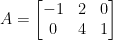
Observations
The example above shows a matrix transformation, since T is defined through multiplying the matrix A and the input vector 
The domain of this transformation is 
If we “plug in” a vector
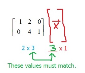
The codomain of this transformation is 
When multiplying a matrix and a vector, the result is determined by the “outer numbers” in our diagram above.

What is happening mathematically to make this true?
If we let 
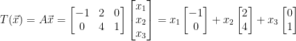
In other words, the image of 

From these two observations, we know that:

That is, T maps vectors in
To find the image of any vector, we just need to multiply
Suppose that we wanted to find the image of the vector 
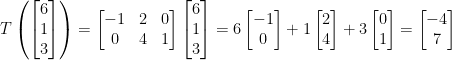
Since 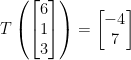

T must be linear
Every matrix transformation is a linear transformation. You can review a proof of this idea here: Proof that every matrix transformation is a linear transformation