Finite Math

Continuously compounding interest formula with examples

Continuously compounding interest is similar to regular compound interest however, interest is not compounded monthly or quarterly but instead, continuously. The continuously compounding interest formula can be used to find the future value of an investment at a given rate or the amount of time it takes to reach a future value given a desired amount. This is commonly taught in college algebra courses or sometimes calculus courses. Below we will look at the formula and some examples of using it.

[adsenseWide]

Examples of finding the future value with the continuously compounding interest formula

We will start with using the formula to calculate the future value of an investment. Then we will look at how to find the time it takes to reach a given future value.

Remember that $e$ is a constant. This is located on your calculator and you should use that instead of an approximation in order to get the most accurate answer.

Example

An investment of $12,000 is invested at a rate of 3.5% compounded continuously. What is its value after 6 years?

Solution

Determine what values are given and what values you need to find. Then, use the formula.

Investment of $12,000 – this is the principle: $P=12000$
Rate 3.5% – remember to write this as a decimal (divide by 100): $r = 0.035$
Value after 6 years: $t = 6$

You are finding the value 6 years in the future, so you are finding $A$, the future value.

$\begin{align}A &= Pe^{rt}\\ &= 12000e^{0.035\times6}\\ &= \bbox[border: 1px solid black; padding: 2px]{14,804.14}\end{align}$

Answer: The value will be $14,804.14 after 6 years.

On your calculator, if you are using a TI83 or TI 84, you should have the following.

The $e$ is located just above $LN$.

Example of finding the time to reach a certain value using the continuously compounding interest formula

In some problems, you may be given a goal value such as $10,000 and asked how long it will take to reach that value given an initial investment. Here, you will use the fact that $\ln(x)$ is the inverse of $e^x$.

Example

An investment of $5,500 is made at a continuously compounding rate of 2%. How many years will it take to reach a value of $15,000?

Solution

Again, review the values you know and what you are trying to find.

Investment of $5,500 so $P = 5500$
Rate 2% so $r = 0.02$
Reach a value of $15,000 – this is the future value so $A = 15000$

We are asked the time, $t$. Now use the formula. Recall the statement above that $\ln(x)$ is the inverse of $e^x$.

$\begin{align}A &= Pe^{rt}\\ 15000 &= 5500e^{0.02\times t}\\ \frac{15000}{5500} &= e^{0.02\times t}\\ \frac{30}{11} &= e^{0.02\times t}\\ \ln\left(\frac{30}{11}\right) &= \ln\left(e^{0.02\times t}\right)\\ \ln\left(\frac{30}{11}\right) &= 0.02t\\ \frac{\ln\left(\frac{30}{11}\right)}{0.02} &= t \\ \bbox[border: 1px solid black; padding: 2px]{50.17} &= t \end{align}$

Answer: About 50 years

Important! Wait as long as possible to round. Rounding early will make your answer off by even a couple of years. Do your work in the calculator. This applies to finding the future value as well.

Continue your study of interest

Now that you have studied the continuously compounding interest formula, you can study other types of interest. Such as:

Simple interest formula and examples

Simple interest is when the interest on a loan or investment is calculated only on the amount initially invested or loaned. This is different from compound interest, where interest is calculated on on the initial amount and on any interest earned. As you will see in the examples below, the simple interest formula can be used to calculate the interest earned, the total amount, and other values depending on the problem.

[adsenseWide]

Examples of finding the interest earned with the simple interest formula

In many simple interest problems, you will be finding the total interest earned over a set period, which is represented as $I$. The formula for this is:

graphic showing the simple interest formula for interest earned

Let’s use an example to see how this formula works. Remember that in the formula, the principal $P$ is the initial amount invested.

Example

A 2-year loan of $500 is made with 4% simple interest. Find the interest earned.

Solution

Always take a moment to identify the values given in the problem. Here we are given:

Time is 2 years: $t = 2$
Initial amount is $500: $P = 500$
The rate is 4%. Write this as a decimal: $r = 0.04$

Now apply the formula:

$\begin{align}I &= Prt \\ &= 500(0.04)(2) \\ &= \bbox[border: 1px solid black; padding: 2px]{40}\end{align}$

Answer: The interest earned is $40.

In this example, the time given was in years, just as in the formula. But what if you are only given a number of months? Let’s use another example to see how this might be different.

Example

A total of $1,200 is invested at a simple interest rate of 6% for 4 months. How much interest is earned on this investment?

Solution

Before we can apply the formula, we will need to write the time of 4 months in terms of years. Since there are 12 months in a year:

$\begin{align}t &= \dfrac{4}{12} \\ &= \dfrac{1}{3}\end{align}$

With this adjusted to years, we can now apply the formula with $P = 1200$ and $r = 0.06$.

$\begin{align}I &= Prt \\ &= 1200(0.06)\left(\dfrac{1}{3}\right) \\ &= \bbox[border: 1px solid black; padding: 2px]{24}\end{align}$

Answer: The interest earned is $24.

If you hadn’t converted here, you would have found the interest for 4 years, which would be much higher. So, always make sure to check that the time is in years before applying the formula.

Important! The time must be in years to apply the simple interest formula. If you are given months, use a fraction to represent it as years.

Another type of problem you might run into when working with simple interest is finding the total amount owed or the total value of an investment after a given amount of time. This is known as the future value, and can be calculated in a couple of different ways.

Finding the future value for simple interest

One way to calculate the future value would be to just find the interest and then add it to the principal. The quicker method however, is to use the following formula.

future value of simple interest formula

You know to use this formula when you are asked questions like “what is the total amount to be repaid” or “what is the value of the investment” -anything that seems to refer to the overall total after interest is considered.

Example

A business takes out a simple interest loan of $10,000 at a rate of 7.5%. What is the total amount the business will repay if the loan is for 8 years?

Solution

The total amount they will repay is the future value, $A$. We are also given that:

$t = 8$
$r = 0.075$
$P = 10\,000$

Using the simple interest formula for future value:

$\begin{align}A &= P(1 + rt)\\ &= 10\,000(1 + 0.075(8)) \\ &= \bbox[border: 1px solid black; padding: 2px]{16\,000}\end{align}$

Answer: The business will pay back a total of $16,000.

This may seem high, but remember that in the context of a loan, interest is really just a fee for borrowing the money. The larger the interest rate and the longer the time period, the more expensive the loan.

Also note that you could calculate this by first finding the interest, I = Prt = 10000(0.075(8)) = $6000, and adding it to the principal of $10000. The final answer is the same using either method.

[adsenseLargeRectangle]

Continue your study of interest

Now that you have studied the simple interest formula, you can learn the more advanced idea of compound interest. Most savings accounts, credit cards, and loans are based on compound instead of simple interest. You can review this idea here:

Compound interest

Compound interest formula and examples

Compound interest is when interest is earned not only on the initial amount invested, but also on any interest. In other words, interest is earned on top of interest and thus “compounds”. The compound interest formula can be used to calculate the value of such an investment after a given amount of time, or to calculate things like the doubling time of an investment. We will see examples of this below.

[adsenseWide]

Examples of finding the future value with the compound interest formula

First, we will look at the simplest case where we are using the compound interest formula to calculate the value of an investment after some set amount of time. This is called the future value of the investment and is calculated with the following formula.

graphic showing the compound interest formula and the definitions of different parts of the formula

Example

An investment earns 3% compounded monthly. Find the value of an initial investment of $5,000 after 6 years.

Solution

Determine what values are given and what values you need to find.

Earns 3% compounded monthly: the rate is $r = 0.03$ and the number of times compounded each year is $m = 12$
Initial investment of $5,000: the initial amount is the principal, $P = 5000$
6 years: $t = 6$

You are trying to find $A$, the future value (the value after 6 years). Now apply the formula with the known values:

$\begin{align}A &= P\left(1 + \dfrac{r}{m}\right)^{mt} \\ &= 5000\left(1 + \dfrac{0.03}{12}\right)^{12 \times 6} \\ &\approx \bbox[border: 1px solid black; padding: 2px]{5984.74}\end{align}$

Answer: The value after 6 years will be $5,984.74.

Important! Be careful about rounding within the formula. You should do as much work as possible in your calculator and not round until the very end. Otherwise your answer may be off by a few dollars.

Let’s try one more example like this before we try some more difficult types of problems.

Example

What is the value of an investment of $3,500 after 2 years if it earns 1.5% compounded quarterly?

Solution

As before, we are finding the future value, A. In this example, we are given:

Value after 2 years: $t = 2$
Earns 3% compounded quarterly: $r = 0.015$ and $m = 4$ since compounded quarterly means 4 times a year
Principal: $P = 3500$

Applying the formula:

$\begin{align}A &= P\left(1 + \dfrac{r}{m}\right)^{mt} \\ &= 3500\left(1 + \dfrac{0.015}{4}\right)^{4 \times 2}\\ &\approx \bbox[border: 1px solid black; padding: 2px]{3606.39}\end{align}$

Answer: The value after 2 years will be $3,606.39.

There are other types of questions that can be answered using the compound interest formula. Most of these require some algebra, and the level of algebra required depends on which variable you need to solve for. We will look at some different possibilities below.

Example of finding the rate given other values

Suppose you were given the future value, the time, and the number of compounding periods, but you were asked to calculate the rate earned. This could be used in a situation where you are taking the amount of home sold for and determining the rate earned, if it is viewed as an investment. Consider the following example.

Example

Mrs. Jefferson purchased an antique statue for $450. Ten years later, she sold this statue for $750. If the statue is viewed as an investment, what annual rate did she earn?

Solution

If we view this as an investment of $P = $450$, then we know that the future value is $A = $750$. This was after $t = 10$ years. Finally, if we assume an annual rate, we will use $m = 1$ and have:

$A = P\left(1 + \dfrac{r}{m}\right)^{mt}$

$750 = 450\left(1 + \dfrac{r}{1}\right)^{1 \times 10}$

This is the same as:

$750 = 450\left(1 + r\right)^{10}$

We are solving for the rate, $r$. We will do this using the following steps.

Divide both sides by 450.

$\dfrac{750}{450} = \left(1 + r\right)^{10}$

Simplify on the left-hand side. But, we need to be careful about rounding, so we will keep the fraction for now.

$\dfrac{5}{3} = \left(1 + r\right)^{10}$

Take the left-hand side to the 1/10th power to clear the power of 10 on the right.

$\left(\dfrac{5}{3}\right)^{\dfrac{1}{10}} = 1 + r$

Calculate the value on the left and solve for $r$.

$\begin{align}1.0524 &= 1 + r \\1.0524 – 1 &= r \\ \bbox[border: 1px solid black; padding: 2px]
{0.0524} &= r\end{align}$

Therefore, Mrs. Jefferson earned an annual rate of 5.24%. Not bad! But there was definitely some more complicated algebra involved. In some cases, you may even have to make use of logarithms. A common situation where you might see this is when calculating the doubling time of an investment at a given rate.

Calculating the doubling time of an investment using the compound interest formula

Regardless of the amount initially invested, you can find the doubling time of an investment as long as you are given the rate and the number of compounding periods. Let’s look at an example and see how this could be done.

Example

How many years will it take for an investment to double in value if it earns 5% compounded annually?

It may seem tough to decide where to start here, as we are only given the rate, $r = 0.05$, and the number of compounding periods, $m = 1$. Note that we are trying to find the time, $t$.

Since we do not know the initial investment, we can simply call it $P$. For this to double, its value would be $2P$ and, using the compound interest formula, we would have:

$A = P\left(1 + \dfrac{r}{m}\right)^{mt}$

$2P = P\left(1 + \dfrac{0.05}{1}\right)^{t}$

This could be written as:

$2P = P\left(1.05\right)^{t}$

Remember that this would only make sense if the amount invested is not zero, so we can divide both side by $P$. This gives:

$2 = \left(1.05\right)^{t}$

To solve for t, we will take the natural log, ln, of both sides. By the laws of logarithms, this will allow us to bring the exponent to the front.

$\ln(2) = t\ln\left(1.05\right)$

Finally, we can divide and then use our calculators to find t.

$\begin{align}t &= \dfrac{\ln(2)}{\ln\left(1.05\right)}\\ &\approx \bbox[border: 1px solid black; padding: 2px]{14.2 \text{ years}}\end{align}$

Answer: It will take a little more than 14 years before the investment will double in value.

The same process could be used to determine when an investment would triple or even quadruple. You would just use a different multiple of $P$ in the first part of the formula.

[adsenseLargeRectangle]

Summary

The compound interest formula is used when an investment earns interest on the principal and the previously-earned interest. Investments like this grow quickly; how quickly depends on the rate and the number of compounding periods. When working with a compound interest formula question, always make note of what values are known and what values need to be found so that you stay organized with your work.

Now that you have studied compound interest, you should also review simple interest and how it is different.

Matrix notation and the size of a matrix

Matrices are used in a variety of different math settings from algebra and linear algebra to finite math. Of course, to be able to work with matrices, you need to understand the notation used and simple (but important) ideas like the size of a matrix.

[adsenseWide]

Elements of a matrix

A matrix is a way of organizing numbers into rows and columns. It may represent a system of equations, a real-life situation, or simply be a matrix of interest all on its own. Matrices are most commonly labeled with capital letters such as A, B, or C. Below, you can see a matrix we will refer to as “matrix A“.

example-of-a-matrix

The numbers within the matrix, are referred to as elements. One way to talk about a specific element is to use a lowercase letter and label it with the row and column of the element.

elements-of-a-matrix

Note that you could also say “5 is the (1,2) entry” and “8 is the (2,3) entry”.

The size of a matrix

The common theme with matrices is “think rows-columns”, and this holds even when discussing the size or dimension of a matrix. If a matrix has 4 rows and 6 columns, we say it is a 4 x 6 matrix (read: four by six).

size-of-a-matrix

Summary

As you study matrices, remember the following ideas:

Elements are referred to by their location in terms of the row, then column.
The size of a matrix is: (number of rows) x (number of columns). For a 2 x 3 matrix, you would say “the size of the matrix is 2 by 3”.

Continue studying matrices

Now that you have reviewed important notation and ideas like the size of a matrix, you are ready to study how to add, subtract, and multiply matrices.

Operations with matrices:

Multiplying matrices with the TI83 or TI84 calculator

Graphing calculators such as the TI83 and TI84 are able to do many different operations with matrices, including multiplication. Here, we will go over the steps needed to multiply two matrices in this type of calculator using the following example.

Table of Contents

Step-by-step process using an example
Common errors
Additional reading

[adsenseWide]

Step-by-step with an example

Find the product of the matrices.

$AB=\left[\begin{array}{ccc}-1 & 5 & -2\\ 3 & 7 & 7\\\end{array}\right]\left[\begin{array}{cc}4 & 0\\ 1 & 1\\ 3 & 9\end{array}\right]$

Step 1: Enter the first matrix into the calculator

To enter a matrix, press [2ND] and $\left[x^{-1}\right]$.

(Note: some older models of the TI83 calculators have a MATRIX button)

multiply-matrices-ti83-ti84-step1-1

Use the right arrow key to go to the EDIT menu.

multiply-matrices-ti83-ti84-step1-2

Press enter to select matrix A.

multiply-matrices-ti83-ti84-step1-3

Type in the size of the matrix and the values by typing each number and pressing [ENTER]. Note that the first matrix is a 2 x 3 matrix (rows by columns).

$A=\left[\begin{array}{ccc}-1 & 5 & -2\\ 3 & 7 & 7\\\end{array}\right]$

multiply-matrices-ti83-ti84-step1-4

Step 2: Enter the second matrix into the calculator

Press [2ND] and $\left[x^{-1}\right]$.

multiply-matrices-ti83-ti84-step2-1

Press the right arrow key to go to the EDIT menu.

multiply-matrices-ti83-ti84-step2-2

Press [2] or highlight 2. [B] and press [ENTER].

multiply-matrices-ti83-ti84-step2-3

Type in the size of the matrix and the values by typing each number and pressing [ENTER]. Note that the second matrix from our example is a 3 x 2 matrix (rows by columns).

$\left[\begin{array}{cc}4 & 0\\ 1 & 1\\ 3 & 9\end{array}\right]$

multiply-matrices-ti83-ti84-step2-4

Step 3: Press [2ND] and [MODE] to quit out of the matrix screen

This will take you to a blank screen. If you skip this step, your calculator may (depending on where your cursor is) try to put matrix A inside of matrix B, causing an error.

Step 4: Select matrix A and matrix B in the NAMES menu to find the product

From the blank screen, press [2ND] and $\left[x^{-1}\right]$ and stay at the NAMES menu.

multiply-matrices-ti83-ti84-step4-1

Press [ENTER] to select matrix [A].

multiply-matrices-ti83-ti84-step4-2

To select matrix [B], go back into the matrix menu by pressing [2ND] and $\left[x^{-1}\right]$.

multiply-matrices-ti83-ti84-step4-3

Press [2] or highlight 2. [B] and press [ENTER].

multiply-matrices-ti83-ti84-step4-4

Press [ENTER] to multiply the matrices.

multiply-matrices-ti83-ti84-step4-5

From here, you have your final answer. We can now write:

$\begin{align} AB &=\left[\begin{array}{ccc}-1 & 5 & -2\\ 3 & 7 & 7\\\end{array}\right]\left[\begin{array}{cc}4 & 0\\ 1 & 1\\ 3 & 9\end{array}\right]
\\ &=\boxed{\left[\begin{array}{cc}-5 & -13\\ 40 & 70\\\end{array}\right]}\end{align}$

Common error: DIM MISMATCH

Suppose that you go through these steps and end up with the following screen.

multiply-matrices-ti83-ti84-dim-mismatch

In this case, you should check two things:

Did you enter the correct matrix information and did you select the correct matrices to multiply?
Is the product defined?

If you entered the matrices correctly, then this error means that the product is undefined. Specifically, if you write out the sizes of the matrices, the inner numbers must match. In the example above, we had a 2 x 3 and a 3 x 2. Notice that the numbers on the inside match, so the product was defined and we were able to find an answer.

However, the product of a 2 x 2 and a 3 x 2 would be undefined since the inner numbers do not match. You would simply write “Undefined” as your answer if you were working a problem like this on an exam or quiz.

To read more about when matrix multiplication is or isn’t defined, see the following link.

When is matrix multiplication defined?

[adsenseLargeRectangle]

Continue your study of matrices and the TI83 / 84 calculator

The following articles have more information about using the calculator with matrices:

Multiplying matrices

While adding or subtracting matrices is relatively straightforward, multiplying matrices is very different from most mathematical operations you have learned beforehand. Here, we will review a nice way to multiply two matrices and some important properties associated with it. You will also learn how to tell when the multiplication is undefined.

[adsenseWide]

Table of contents:

Multiplying two matrices: “rows hit columns” (animation of this)
Matrix multiplication is not always defined
Matrix multiplication is not commutative
Examples of multiplying matrices
Summary of properties

Multiplying two matrices: “rows hit columns”

To understand the general pattern of multiplying two matrices, think “rows hit columns and fill up rows”. Consider the following example.

The first row “hits” the first column, giving us the first entry of the product. Notice that since this is the product of two 2 x 2 matrices (number of rows and columns), the result will also be a 2 x 2 matrix. We will look at how the size of the matrix affects this later in the article.
matrix-multiplication1

Now, the first row “hits” the second column, filling up the row of the product.
matrix-multiplication2

Having run out of columns to “hit”, we now work with the second row.
matrix-multiplication3

There is one last entry to calculate. The second row will now “hit” the second column.

matrix-multiplication4

Finally, we just need to complete the arithmetic to get our final answer.
matrix-multiplication5

An animation of this process

You can see an animation of this process here. There is no sound – so don’t worry about finding your headphones!

We will see a couple more examples shortly, but first, we need to discuss how the size of a matrix affects the result when multiplying. In fact, there are cases where due to the size of the matrix, the multiplication is undefined.

Matrix multiplication is not always defined

When multiplying matrices, the size of the two matrices involved determines whether or not the product will be defined. You can also use the sizes to determine the result of multiplying the two matrices. Recall that the size of a matrix is the number of rows by the number of columns. The matrices above were 2 x 2 since they each had 2 rows and 2 columns.

matrix-product-is-defined

As you can see, the sizes of the matrices do not have to be the same, you just need the middle two numbers to match when you write the sizes side by side. Otherwise, the product is undefined.

matrix-product-is-not-defined

Think about this: if a matrix A is 3 x 4, for example, then the product of A and itself would not be defined, as the inner numbers would not match. This is just one example of how matrix multiplication does not behave in the way you might expect.

Matrix multiplication is not commutative

You know from grade school that the product (2)(3) = (3)(2). It doesn’t matter which order you multiply the numbers in, the result is the same. This does not work in general for matrices. Only in special cases can you say that AB = BA. So, in general, you should assume that they are not equal. It can even be the case that AB is defined, while BA is not defined!

not-commutative

Even if the product is defined, again, it is unlikely the results will be the same for AB and BA.

not-commutative2

Examples of multiplying matrices

Now that we have seen some of the important properties of matrix multiplication, let’s work through a couple of examples.

Example

Find the product AB where:
$A = \left[\begin{array}{cc} -5 & 3\\ -4 & -1\\ \end{array}\right]$
and
$B = \left[\begin{array}{cc} 1 & -1\\ 2 & 6\\ \end{array}\right]$

Solution

Remember that rows hit columns, and fill up rows. Here, the matrices are each 2 x 2 and so the result will be a 2 x 2 matrix.

$\begin{align} AB &= \left[\begin{array}{cc} -5 & 3\\ -4 & -1\\ \end{array}\right] \left[\begin{array}{cc} 1 & -1\\ 2 & 6\\ \end{array}\right]\\ &= \left[\begin{array}{cc} -5(1) + 3(2) & -5(-1) + 3(6)\\ -4(1) +(-1)(2) & (-4)(-1)+(-1)(6)\\ \end{array}\right]\\ &= \boxed{\left[\begin{array}{cc} 1 & 23\\ -6 & -2\\ \end{array}\right]}\end{align}$

Example

Find the product AB where:

$A = \left[\begin{array}{cccc} -2 & -1 & 0 & 0 \\ 1 & 2 & 1 & 1\\ \end{array}\right]$
and
$B = \left[\begin{array}{cccc} 3 & 1 & 1 & 2 \\ -1 & -1 & 0 & 1\\ \end{array}\right]$

Solution

Here, we have a 2 x 4 matrix multiplied by a 2 x 4 matrix. The inner numbers of these sizes do not match, therefore:

$\boxed{AB \text{ is undefined}}$

Example

Find the product AB where:
$A = \left[\begin{array}{cc} 1 & 2\\ -2 & 0\\ 3 & 1\\\end{array}\right]$

and
$B = \left[\begin{array}{cc} 4 & 0\\ 0 & 1\\ \end{array}\right]$

Solution

This is the product of a 3 x 2 matrix and a 2 x 2 matrix. The inner numbers match, so the product is defined. The result will be a 3 x 2 matrix.

$\begin{align} AB &= \left[\begin{array}{cc} 1 & 2\\ -2 & 0\\ 3 & 1\\\end{array}\right]\left[\begin{array}{cc} 4 & 0\\ 0 & 1\\ \end{array}\right]\\ &= \left[\begin{array}{cc} 1(4) + 2(0) & 1(0) + 2(1)\\ -2(4) + 0(0) & -2(0) + 0(1)\\ 3(4) + 1(0) & 3(0) + 1(1)\\\end{array}\right]\\ &= \boxed{\left[\begin{array}{cc} 4 & 2\\ -8 & 0\\ 12 & 1\\\end{array}\right]}\end{align}$

[adsenseLargeRectangle]

Summary

Remember the following anytime you are multiplying two or more matrices.

Rows hit columns and fill up rows.
Matrix multiplication is not always defined – check the matrix sizes first!
Matrix multiplication is not commutative, in general.

Adding and subtracting matrices, and multiplying a matrix by a constant

When multiplying a matrix by a scalar (a constant or number), or adding and subtracting matrices, the operations are done entry by entry. Let’s look at each operation separately to see how that works.

Table of Contents

Adding matrices
Subtracting matrices
Multiplying a matrix by a constant (scalar multiplication)
Combining addition, subtraction, and scalar multiplication

[adsenseWide]

Adding matrices

To add two matrices, add corresponding entries, as shown below. Notice that you need the matrices to be the same size in order for this to make sense.
Image of two matrices being added. Since the matrices are the same size, the corresponding entries can be added.

If the matrices are different sizes, the addition is undefined.
Image of adding matrices of two different sizes. This is not possible, so the sum is undefined.

Subtracting matrices

Subtracting matrices works in the same way. You can subtract entry by entry.

Image of subtracting two matrices. Since they are the same size, corresponding entries are subtracted.

Just as with addition, this would be undefined if the matrices were different sizes. In that situation, your answer would simply be “undefined”.

Multiplying a matrix by a constant (scalar multiplication)

The multiplication of a matrix by a constant or number (sometimes called a scalar) is always defined, regardless of the size of the matrix. You just need to make sure that each entry in the matrix is multiplied by the number.

Multiplication of a matrix and a scalar. Each entry in the matrix is multiplied.

Combining operations

In some questions, you might be asked to combine addition, subtraction, and multiplication by a constant. Here, we will look at a couple of examples to make sure you know how to approach these.

Example

Find $-2A + B$ for:

$A= \left[\begin{array}{cc} -4 & 1\\ 2 & -2\\ \end{array}\right]$ and $B= \left[\begin{array}{cc} 9 & -4\\ 0 & 8\\ \end{array}\right]$

Remember to multiply each entry by the constant and to work entry by entry when adding.

$\begin{align} -2A + B &= 2\left[\begin{array}{cc} -4 & 1\\ 2 & -2\\ \end{array}\right] + \left[\begin{array}{cc} 9 & -4\\ 0 & 8\\ \end{array}\right]\\ &= \left[\begin{array}{cc} -2 \times -4 & -2 \times 1\\ -2 \times 2 & -2 \times -2\\ \end{array}\right] + \left[\begin{array}{cc} 9 & -4\\ 0 & 8\\ \end{array}\right]\\ &= \left[\begin{array}{cc} 8 & -2\\ -4 & 4\\ \end{array}\right] + \left[\begin{array}{cc} 9 & -4\\ 0 & 8\\ \end{array}\right]\\ &= \left[\begin{array}{cc} 8 + 9 & -2 + (-4) \\ -4 + 0 & 4 + 8\\ \end{array}\right]\\ &= \boxed{\left[\begin{array}{cc} 17 & -6 \\ -4 & 12\\ \end{array}\right]}\end{align}$

This also works when you have more than two matrices, as seen in the next example.

Example

Find $A – 3B + 2C$ for:

$A= \left[\begin{array}{cc} 1 & 1\\ 0 & 0\\ \end{array}\right]$ , $B= \left[\begin{array}{cc} 2 & 1\\ 1 & 4\\ \end{array}\right]$, and $C= \left[\begin{array}{cc} 5 & 2\\ 3 & 0\\ \end{array}\right]$

$\begin{align} A – 3B + 2C &= \left[\begin{array}{cc} 1 & 1\\ 0 & 0\\ \end{array}\right] – 3\left[\begin{array}{cc} 2 & 1\\ 1 & 4\\ \end{array}\right] + 2\left[\begin{array}{cc} 5 & 2\\ 3 & 0\\ \end{array}\right]\\ &= \left[\begin{array}{cc} 1 & 1\\ 0 & 0\\ \end{array}\right] – \left[\begin{array}{cc} 3\times2 & 3\times1\\ 3\times1 & 3\times4\\ \end{array}\right] + \left[\begin{array}{cc} 2\times5 & 2\times2\\ 2\times3 & 2\times0\\ \end{array}\right]\\ &= \left[\begin{array}{cc} 1 & 1\\ 0 & 0\\ \end{array}\right] – \left[\begin{array}{cc} 6 & 3\\ 3 & 12\\ \end{array}\right] + \left[\begin{array}{cc} 10 & 4\\ 6 & 0\\ \end{array}\right]\\ &= \left[\begin{array}{cc} 1 – 6 + 10 & 1 – 3 + 4\\ 0 – 3 + 6 & 0 – 12 + 0\\ \end{array}\right]\\ &= \boxed{\left[\begin{array}{cc} 5 & 2\\ 3 & – 12\\ \end{array}\right]}\end{align}$

Summary

Remember the following for operations on matrices:

To add or subtract, go entry by entry.
Addition and subtraction are only defined if the matrices are the same size.
Scalar multiplication is always defined – just multiply every entry of the matrix by the scalar.

[adsenseLargeRectangle]

Continue your study of matrix operations

Next: Multiplying matrices

Combinations on the TI83 or TI84 calculator

In counting, combinations are used to find the number of ways a selection can be made, when order doesn’t matter. In this article, we will see how to use a calculator to find combinations. Let’s use an example to see how this works!

[adsenseWide]

You are taking a week-long trip and decide to bring 4 books from your collection of 25 books. How many different groups of 4 books can be selected from your collection?

Here, you only care about which four books are chosen, not the order. Thus, a combination can be used to answer this question: C(25, 4) or “25 choose 4”.

Step 1: Type in the first number

In this case, the first number is 25.

combinations-on-calculator-step1

Step 2: Press [MATH] and go to the PRB menu

You can use the right arrow to select the menu at the top.

combinations-on-calculator-step2

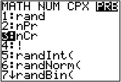
Step 3: Select 3 nCr and press [ENTER]

To select 3: nCr, you can either highlight the 3 or just press the 3 button.

combinations-on-calculator-step3-5

combinations-on-calculator-step3

Step 4: Type the second number and press [ENTER]

We are finding C(25,4), so the second number is 4.

combinations-on-calculator-step4

From this, we see that there are C(25, 4) = 12,650 different groups of 4 books that could be selected. This may seem like the answer is too large, but if you start thinking about how only one book needs to be different for the group of 4 books to be considered a different group, it begins to make more sense.

Other methods for calculating combinations

You can also use the formula to calculate a combination. You can review this, and more about combinations in general, below.

Counting with combinations

Combinations are a way of counting how many ways there are to select an object when order doesn’t matter. For example, suppose that you are selecting 3 people from a group of 15 to take a survey. All 3 selected are taking the same survey, and so the order they are selected in isn’t important.

[adsenseWide]

Notation for combinations

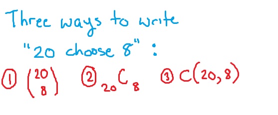
Before we get into some examples, it is important to note that there are three common ways to write a combination. Suppose that we are selecting 8 objects from a basket of 20, and the order isn’t important. The number of ways this can be done would be calculated with a combination “20 choose 8”. This can be written as:

notation-for-combinations

Each of these has the same value, they are just different ways of representing the combination. For this article, we will use the third: C(20,8).

Formula for combinations

Combinations can be calculated using either the formula or using a calculator. The formula uses factorials (the exclamation point). Remember that factorials are where you count down and multiply. For example, 4! = 4 x 3 x 2 x 1 = 24.
combinations-formula
Now, we can look at a few examples of counting with combinations.

Examples

For each of these examples, pay close attention to how it is determined that order is not important. Remember that if order was important, we would use permutations instead.

Example

Jacob’s manager asks him to select 3 shifts from the 7 shifts available next week. How many different selections of three shifts are possible?

In this problem, it doesn’t matter which shift Jacob selected first or second, as he will be working the three selected shifts regardless. Therefore, the answer is: C(7,3).

$C(7, 3) = \dfrac{7!}{3!(7 - 3)!}$

$= \dfrac{7!}{3!(4!)}$

$= \dfrac{7 \times 6 \times 5 \times \overbrace{4 \times 3 \times 2 \times 1}^{\text{cancel}}}{(3 \times 2 \times 1)(\underbrace{4 \times 3 \times 2 \times 1}_{\text{cancel}})}$

$= \dfrac{7 \times \overbrace{6}^{\text{cancel}} \times 5}{\underbrace{3 \times 2 \times 1}_{\text{cancel}}}$

$= 7 \times 5$

$= \boxed{35}$

Notice how many terms we were able to cancel out. This will happen with every combination problem, no matter how large the numbers are. Cancelling out at least some of the terms is always nice, as then it is easier to input in the calculator (or, like in the case above, you may not even need a calculator!)

Example

In how many ways can a committee of 6 be selected from a group of 35 students?

When selecting a committee, it is understood that you are simply selecting a group of people to discuss or work on a problem – the order in which they are selected isn’t important since if someone is selected, they are on the committee whether they were selected first or last. Therefore, we can count this using combinations: C(35, 6).

$C(35, 6) = \dfrac{35!}{6!(35 - 6)!}$

$= \dfrac{35!}{6!(29!)}$

$= \dfrac{35 \times 34 \times 33 \times 32 \times 31 \times 30 \times \overbrace{29 \times 28 \times 27 \times \cdots \times 1}^{\text{cancel}}}{(6 \times 5 \times 4 \times 3 \times 2 \times 1)(\underbrace{29 \times 28 \times 27 \times \cdots \times 1}_{\text{cancel}})}$

$= \dfrac{35 \times 34 \times 33 \times 32 \times 31 \times \overbrace{30}^{\text{cancel}}}{(\underbrace{6 \times 5}_{\text{cancel}} \times 4 \times 3 \times 2 \times 1)}$

$= \dfrac{35 \times 34 \times 33 \times 32 \times 31}{4 \times 3 \times 2 \times 1}$

$= \boxed{1\,623\,160}$

This number may seem very large, but you would be surprised how many different choices there are when the group you are selecting from is large. It is very common in counting problems to come across very large answers like this.

Combinations on the calculator

You can also use a calculator to calculate combinations. To see how to use a TI83 or 84 calculator for this, see the article below.

Combinations on the TI83 or TI84 calculator

Row reduction with the TI83 or TI84 calculator (rref)

Row reducing a matrix can help us find the solution to a system of equations (in the case of augmented matrices), understand the properties of a set of vectors, and more. Knowing how to use row operations to reduce a matrix by hand is important, but in many cases, we simply need to know what the reduced matrix looks like. In these cases, technology like a graphing calculator is a great tool to use!

[adsenseWide]

We will go through the steps using this matrix:

3x3-matrix

Step 1: Go to the matrix menu on your calculator.

Press [2nd][x^-1] to enter the matrix menu. Note that some older calculators have a button that simply says [MATRX]. Press the right arrow until you are under the EDIT menu.

Press [ENTER] and you can now edit matrix A.

Step 2: Enter your matrix into the calculator.

The first information you are asked is the size of the matrix. This matrix has 3 rows and 3 columns, so it is a 3 x 3 matrix. Type these numbers, pressing [ENTER] after each.

edit-matrix-A-3x3-ti83-ti84

Now you can enter each number by typing it and pressing [ENTER].

matrix-entered-into-ti83-ti84

Step 3: Quit out of the matrix editing screen.

This is a strange step, but if we don’t do it, the calculator tries to put a reduced matrix INSIDE of this matrix. It’s a bug for sure, but one we can work around.

Press [2nd] and then [MODE] to quit. You will end up at a blank screen.

Step 4: Go to the matrix math menu.

Press [2nd][X^-1] to enter the matrix menu again, but this time go over to MATH.

$matrix-math-menu-ti83-ti84$

Scroll down to “rref” (reduced row echelon form) and press [ENTER].

rref-ti83-ti84

Step 5: Select matrix A and finally row reduce!

To select matrix A, you need to go back into the matrix menu by pressing [2nd][x^-1] but stay under the NAMES menu.

Now press [ENTER] to select matrix A.

rref-A-ti83-ti84

Close your parentheses by pressing [ ) ] and then pressing [ENTER] to get the reduced matrix.

(note: you don’t have to close the parentheses for this to work, but it is a good habit – or maybe just not closing parentheses drives me crazy… one of those..).

rref-reduced-A-ti83-ti84

Interesting! This matrix turns out to be row equivalent to the identity matrix. If you are currently studying linear algebra, you know that this is a useful fact to know about a matrix. There are many properties that are now automatically true for our matrix A!

Either way, we are done. We now have row reduced matrix A.

Fractions vs. Decimals

One thing that can happen when you row reduce, is that you end up with messy decimals. With one additional step, you can convert these to fractions. So, suppose we reduced a matrix and ended up with the following:

decimals-after-reducing-matrix-ti83-ti84

Before pressing any other buttons, press [MATH] and then select >FRAC by pressing [ENTER].

$math-frac-ti83-ti84$

$math-frac-matrix-ti83-ti84$

Now press [ENTER] to get a reduced matrix with fractions instead of decimals.

$math-frac-matrix-ti83-ti84-2$

This is much better! You will want to use this for most mathematical problems, as the fractions are exact values and the decimals before were approximations.

[adsenseLargeRectangle]

Additional Reading

Now that you are comfortable with row reduction using the calculator, you can learn how to multiply matrices with the TI83/84 or find the inverse with your calculator as well!