Finite Math

Row operations

Row operations are calculations we can do using the rows of a matrix in order to solve a system of equations, or later, simply row reduce the matrix for other purposes. There are three row operations that we can perform, each of which will yield a row equivalent matrix. This means that if we are working with an augmented matrix, the solution set to the underlying system of equations will stay the same.

[adsenseWide]

The row operations

In the following examples, the symbol ~ means “row equivalent”.

Swap two rows

When working with a system of equations, the order you write the questions doesn’t affect the solution. Since an augmented matrix represents a system of equations, with each row being an equation, we can swap two rows.

row-operations-swap-rows

Notice the notation with the double arrow. When you are performing row operations, use notation like this to keep track of what you did. It is very easy to have an arithmetic mistake, and if this happens, this notation let’s you go back and find it easily.

The formal notation for this row operation (as used in some books) would be: $R_1 \leftrightarrow R_3$ .

Multiply a row by a nonzero constant

There will be times when it will be useful to multiply a row by something like 2 or 1/3. Doing this will not change the solution to the underlying system of equations since multiplying any equation by a nonzero constant results in an equivalent equation (as long as you multiply BOTH sides of the equation).

row-operations-multiply-a-row-by-constant

In this example, each entry in row 2 was multiplied by the constant. A fair question here would be “Why would you do that row operation?”. We will get into that when we talk about Gauss Jordan elimination and row reduction, but for now, I chose multiplying row 2 by 3 just for the sake of showing you how it would work.

The formal notation for this particular row operation: $3R_2 \rightarrow R_2$ . (think: multiply row 2 by 3 and put it back where the original row 2 was)

Multiply a row by a nonzero constant and add it to another row

Think back to when you first learned how to solve systems of equations. You likely learned how to eliminate a variable by multiplying one equation by a number and then adding the two equations. We can translate that same idea into a row operation.

row-operations-adding-rows

Notice that all the work happened in row 2. Because of this, our shorthand notation has $-5R_1$ next to row 2. To do the actual row operation, we took each value in row 1, multiplied it by –5 and then added it to the corresponding entry in row 2.

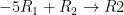
The formal notation for this would be: $-5 R_1 + R_2 \rightarrow R2$ . (the arrow points to where all the work will go)

The big picture

The last example shows the true power of row operations. By picking to add $-5R_1$ to row 2, we eliminated $x_1$ in the 2nd equation. If we continued this process and did similar row operations for other variables, then we should be able to eliminate the variables in a way as to see the solution to the underlying system. In fact, this will be exactly what we will study when talking about Gauss Jordan elimination and row reduction.

Augmented matrices and systems of linear equations

You can think of an augmented matrix as being a way to organize the important parts of a system of linear equations. These “important parts” would be the coefficients (numbers in front of the variables) and the constants (numbers not associated with variables).

[adsenseWide]

Writing the augmented matrix for a system

Let’s look at two examples and write out the augmented matrix for each, so we can better understand the process. The key is to keep it so each column represents a single variable and each row represents a single equation. The augment (the part after the line) represents the constants.

Example

Write the augmented matrix for the system of equations:
$\begin{array}{l}3x_1 + 5x_2 – x_3 = 10\\ x_1 + 4x_2 + x_3 = 7\\ 9x_1 + 2x_3 = 1\\ \end{array}$

Solution

There are three variables, and so we will need a column for each. Be careful – notice that the last equation doesn’t have an $x_2$. That will be represented with a 0.

Augmented matrix for the system; each column represents the coefficients for the variables and each row represents an equation. Row 1 is 3 5 -1 10, Row 2 is 1 4 1 7, and row 3 is 9 0 2 1. The 10, 7, and 1 each represent the constants from the equations.

Example

Write the augmented matrix for the system of equations:

$\begin{array}{l} x_1 – 2x_2 + 8x_3 + x_4 + x_5 = 2\\ 3x_1 – x_2 + x_3 + 2x_4 + 2x_5 = -3\\ \end{array} $

Solution

Even though this is not the type of system we are used to seeing in our usual algebra classes, we can still write an augmented matrix to represent it. The augmented matrix for this system would be:

Augmented matrix for example 2. The first row is 1 -2 8 1 1 2, for the coefficients and constants from the first equation. The second row is 3 -1 1 2 2 -3 for the constants and coefficients from the second equation.

Common Questions

Does the order that I write the rows in matter?

No. In algebra, when you were solving a system like $3x + y = 5$ and $2x + 4y = 7$, it didn’t matter if you wrote one equation first or second. The solution to the problem didn’t change. The same is true when you have more than two equations. Since each row represents an equation, the order that you write the rows in doesn’t matter.

What is this used for?

Putting a system of equations in this form will allow us to use a new idea called row operations to find its solution (if one exists), describe the solution set (when there are infinitely many solutions), and more. Row operations can help us organize a way to do this regardless of how many variables or how many equations we are given. This will be studied in later articles.

Counting with the multiplication rule

Counting is a really tough area of mathematics, but is also really important for understanding real life applications and, later, for finding probabilities. In this article, we will study one particular method used in counting: the multiplication rule.

[adsenseWide]

The multiplication rule

Imagine you are trying to guess someone’s password. If you know that the password is made up of 5 letters or numbers, we can imagine that you simply guess all 5 at once. But, we could also imagine that you guess the first letter or number, then the second, then the third, and so on. In the end, the result is the same but the way we think about it is different.

If you can think of a process in steps like this, then we can apply the multiplication rule. In order to find the total number of possible passwords, we first think of how many possibilities there are for the first character, how many for the second, and so on. We then multiply these to find the total number of possibilities.

Example – Passwords

A password is 5 characters long and is made up of letters and numbers. How many different passwords like this are possible?

We will think about the number of possibilities for each character individually.

We know the password is made up of letters and numbers. Some observations about this:

There are 26 letters in the alphabet.
There are 10 possible numbers for any for any character: 0, 1, 2, 3, 4, 5, 6, 7, 8, 9
In a password, uppercase and lowercase letters are considered different, so there are 26 + 26 = 52 possible letters for any character.

For the first character, this means there are a total of 10 + 52 = 62 possibilities.

For the next character, we still have 62 possibilities. There was no indication that the password can’t use the same letter or number twice. In fact, there are the same number of possibilities for each character. Filling this in and applying the multiplication rule we have:

Example – passwords revisited

A password is 5 characters long, is made up of letters and numbers, and has no repeated characters. How many different passwords like this are possible?

This question is almost identical to the first one, except for one part: no repeated characters. Pay attention to wording like this!!

This tells you that after you have used one number or letter, you can’t use it again. So the number of choices for the first character is still 62. But now, you have used 1 of the characters, so there are only 61 to choose from for the next. This pattern continues after each choice is made.

Example – buying sandwiches

A deli let’s customers build their own sandwich. They can select from three types of bread (wheat, white, and rye), two types of cheese (american or provolone), four types of meat (turkey, roast beef, ham, and salami) and a sauce (regular mayo, hot mayo, bbq). Using these ingredients, how many different sandwiches are possible?

Applications

Really, you could think of any counting problem as a true application problem – if you have ever seen a commercial that says “over 15,000 different varieties” of something like that, then you have seen counting in use!

When you think about counting, there are some other interesting problems that come up. For example, how many 4 digit bank pin codes are possible? (answer: 10,000 – can you use the multiplication rule to figure out why?) Using another rule called the Pigeonhole Principle, we can say that this means that in any group of more than 10,000 people, at least two MUST share the same pin number. But, this assumes people pick codes randomly – so how true is that? I explore that on my personal blog in the following article: pin codes and the birthday problem.