Linear Algebra

Linearly independent vectors with examples


A set of vectors is linearly independent when none of the vectors can be written as a linear combination of the other vectors. This applies to vectors in \(\mathbb{R}^n\) for any \(n\) or vector spaces like the polynomial spaces. The more formal definition along with some examples are reviewed below. We will see how to determine if a set of vectors is linearly independent or dependent using the definition or theorems.

[adsenseWide]

The formal definition of linear independence

A set of vectors is linearly independent if and only if the equation:

\(c_1\vec{v}_1 + c_2\vec{v}_2 + \cdots + c_k\vec{v}_k = \vec{0}\)

has only the trivial solution. What that means is that these vectors are linearly independent when \(c_1 = c_2 = \cdots = c_k = 0\) is the only possible solution to that vector equation.

If a set of vectors is not linearly independent, we say that they are linearly dependent. Then, you can write a linear dependence relation showing how one vector is a combination of the others.

Examples of determining when vectors are linearly independent

Let’s stick to \(\mathbb{R}^n\) for now and look at how to determine if those vectors are linearly independent or not. Let’s get into the first example!

Example

Are the vectors \(\vec{v}_1 = \left[\begin{array}{c} 1\\ 4\\ 0\\\end{array}\right], \vec{v}_2 = \left[\begin{array}{c} 10\\ 2\\ 1\\\end{array}\right], \vec{v}_3 = \left[\begin{array}{c} -5\\ 0\\ 6\\\end{array}\right]\) linearly independent?

Solution

This is asking “does the following equation have only the trivial solution (all 0’s)?”

\(c_1\left[\begin{array}{c} 1\\ 4\\ 0\\\end{array}\right] + c_2\left[\begin{array}{c} 10\\ 2\\ 1\\\end{array}\right] + c_3\left[\begin{array}{c} -5\\ 0\\ 6\\\end{array}\right] = \left[\begin{array}{c} 0\\ 0 \\ 0 \\ \end{array}\right]\)

Every vector equation (in the real spaces) is equivalent to a matrix equation and an augmented matrix. An augmented matrix would be most useful here. We will need to row reduce using the calculator.

\(\left[\begin{array}{ccc|c} 1 & 10 & -5 & 0\\ 4 & 2 & 0 & 0\\ 0 & 1 & 6 & 0\\ \end{array}\right] \sim \left[\begin{array}{ccc|c} 1 & 0 & 0 & 0\\ 0 & 1 & 0 & 0\\ 0 & 0 & 1 & 0\\ \end{array}\right] \)

As you can see from this matrix, the solution to the vector equation (since it is equivalent) is \(c_1 = c_2 = c_3 = 0\), the trivial solution. We know this is the only solution because there are no free variables in the equation. Since the only solution to the vector equation is the trivial solution, these vectors are linearly independent.

Example

Are the vectors \(\vec{v}_1 = \left[\begin{array}{c} 6\\ 2\\ 9\\ 1 \\\end{array}\right], \vec{v}_2 = \left[\begin{array}{c} 12\\ 4\\ 18\\ 2\\\end{array}\right], \vec{v}_3 = \left[\begin{array}{c} 8\\ 0\\ 0\\ 0\\\end{array}\right], \vec{v}_4 = \left[\begin{array}{c} -2\\ 1\\ 1\\ 5\\\end{array}\right]\) linearly independent?

Solution

You may notice that vector 2 is a multiple of vector 1. This means the vectors are not linearly independent but instead are linearly dependent. But how would this look in a matrix? Let’s take a look.

\(\left[\begin{array}{cccc|c} 6 & 12 & 8 & -2 & 0\\ 2 & 4 & 0 & 1 & 0\\ 9 & 18 & 0 & 1 & 0 \\ 1 & 2 & 0 & 5 & 0 \\ \end{array}\right] \sim \left[\begin{array}{cccc|c} 1 & 2 & 0 & 0 & 0\\ 0 & 0 & 1 & 0 & 0\\ 0 & 0 & 0 & 1 & 0 \\ 0 & 0 & 0 & 0 & 0 \\ \end{array}\right]\)

We have a column (column 2) which is not a pivot column. This means that we have a free variable in the vector equation underlying this matrix. That means there are infinitely many solutions i.e., nontrivial solutions (solutions where the constants are not all zero). Therefore these vectors are linearly dependent.

Properties of linearly independent vectors

While you can always use an augmented matrix in the real spaces, you can also use several properties of linearly independent vectors. We will use these without proofs, which can be found in most linear algebra textbooks.

  • A set with one vector is linearly independent.
  • A set of two vectors is linearly dependent if one vector is a multiple of the other.

    \(\left[\begin{array}{c} 1 \\ 4\\ \end{array}\right]\) and \(\left[\begin{array}{c} -2 \\ -8\\ \end{array}\right]\) are linearly dependent since they are multiples.

    \(\left[\begin{array}{c} 9 \\ -1\\ \end{array}\right]\) and \(\left[\begin{array}{c} 18 \\ 6\\ \end{array}\right]\) are linearly independent since they are not multiples.

  • Any set containing the zero vector is a linearly dependent set.
    This is because you can write any constant in front of the zero vector to get a nontrivial solution to the vector equation from the definition.

    The vectors:

    \(\left[\begin{array}{c} 5 \\ 0\\ \end{array}\right]\), \(\left[\begin{array}{c} 2 \\ 6\\ \end{array}\right]\), \(\left[\begin{array}{c} 0 \\ 0\\ \end{array}\right]\)

    are linearly dependent because the set contains the zero vector.

  • Any set where one vector is a linear combination of the others is linearly dependent.
    We saw this above. It is true for any size set.

  • A set with more vectors than entries in the vectors is linearly dependent.
    The vectors:

    \(\left[\begin{array}{c} 2 \\ 6\\ \end{array}\right]\), \(\left[\begin{array}{c} 1 \\ 1\\ \end{array}\right]\), \(\left[\begin{array}{c} -1 \\ 5\\ \end{array}\right]\)

    are linearly dependent because there are 3 vectors but each vector has 2 entries.

    Where do linearly independent vectors come into play?

    One big area where you will work with linearly independent vectors is when talking about the basis of a vector space. This is a linearly independent set that spans the vector space.

    Continue your study of linear algebra topics: https://www.mathbootcamps.com/linear-algebra-guides-and-articles/

The column space of a matrix

The column space of a matrix is the span, or all possible linear combinations, of its columns.

Let’s look at some examples of column spaces and what vectors are in the column space of a matrix. Note that since it is the span of a set of vectors, the column space is itself a vector space.

Example and discussion

[adsenseWide]

Notation

We denote the column space of a matrix as \(\text{Col }A\).

Example with a 3 x 4 matrix

Let \(A = \left[\begin{array}{cccc} -2 & -1 & 1 & 5\\ 6 & 10 & 0 & -3\\ 7 & 0 & 1 & 0\\ \end{array}\right]\)

The column space of this matrix is:

\(\text{Span}\{\left[\begin{array}{c} -2 \\6 \\ 7\\ \end{array}\right],\left[\begin{array}{c} -1 \\10 \\ 0\\ \end{array}\right],\left[\begin{array}{c} 1 \\0 \\ 1\\ \end{array}\right],\left[\begin{array}{c} 5 \\-3 \\ 0\\ \end{array}\right]\}\)

What are some vectors in the columns space of A?

Any linear combination of the columns are in the columns space since that is the definition of span from above. This means every column is in the column space. For example, the second column can be written as:

\(\left[\begin{array}{c} -1 \\10 \\ 0\\ \end{array}\right] = (0)\left[\begin{array}{c} -2 \\6 \\ 7\\ \end{array}\right] + (1)\left[\begin{array}{c} -1 \\10 \\ 0\\ \end{array}\right] + (0)\left[\begin{array}{c} 1 \\0 \\ 1\\ \end{array}\right] + (0)\left[\begin{array}{c} 5 \\-3 \\ 0\\ \end{array}\right]\)

The zero vector is in the column space. This can be shown by letting all the weights equal zero. Remember that this must be the case in order for this to be a vector space (well a subspace but we will get that in a minute, anyway any subspace of a vector space is a vector space in its own right.)

\(\left[\begin{array}{c} 0 \\0 \\ 0\\ \end{array}\right] = (0)\left[\begin{array}{c} -2 \\6 \\ 7\\ \end{array}\right] + (0)\left[\begin{array}{c} -1 \\10 \\ 0\\ \end{array}\right] + (0)\left[\begin{array}{c} 1 \\0 \\ 1\\ \end{array}\right] + (0)\left[\begin{array}{c} 5 \\-3 \\ 0\\ \end{array}\right]\)

Finally, to reiterate, any linear combination of these columns are in the column space. So we can use any weights to find such a vector. For example:

\(\left[\begin{array}{c} 1 \\43 \\ 9\\ \end{array}\right] = (1)\left[\begin{array}{c} -2 \\6 \\ 7\\ \end{array}\right] + (4)\left[\begin{array}{c} -1 \\10 \\ 0\\ \end{array}\right] + (2)\left[\begin{array}{c} 1 \\0 \\ 1\\ \end{array}\right] + (1)\left[\begin{array}{c} 5 \\-3 \\ 0\\ \end{array}\right]\)

So:

\(\left[\begin{array}{c} 1 \\43 \\ 9\\ \end{array}\right] \in \text{Col }A\)

What space is the column space a subspace of?

When you are determining this, count the number of entries in the vectors that make up the columns. Each vector has three entries, so the vectors are in \(\mathbb{R}^3\). That means any linear combination of them is in the same space. Thus the column space is a subspace of \(\mathbb{R}^3\) in this example.

Other spaces associated with matrices

With a matrix, you can also talk about the row space and the null space.

The identity matrix and its properties

The identity matrix is a square matrix that has 1’s along the main diagonal and 0’s for all other entries. This matrix is often written simply as \(I\), and is special in that it acts like 1 in matrix multiplication. In this lesson, we will look at this property and some other important idea associated with identity matrices.

[adsenseWide]

The identity matrix is always a square matrix

While we say “the identity matrix”, we are often talking about “an” identity matrix. For any whole number \(n\), there is a corresponding \(n \times n\) identity matrix. These matrices are said to be square since there is always the same number of rows and columns.

a 2 x 2 and a 3 x3 identity matrix

To prevent confusion, a subscript is often used. So in the figure above, the \(2 \times 2\) identity could be referred to as \(I_2\) and the \(3 \times 3\) identity could be referred to as \(I_3\).

Multiplying any matrix by the identity results in the matrix itself

When working with matrix multiplication, the size of a matrix is important as the multiplication is not always defined. Therefore for an \(m \times n\) matrix \(A\), we say:

multiplication property with the identity matrix

This shows that as long as the size of the matrix is considered, multiplying by the identity is like multiplying by 1 with numbers. For example, consider the following matrix.

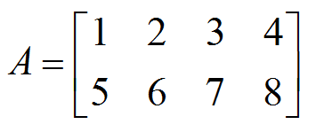
example of a 2 by 4 matrix

This is a \(2 \times 4\) matrix since there are 2 rows and 4 columns. You can verify that \(I_2 A = A\):

left hand multiplication by the identity

and \(A I_4 = A\):

right hand multiplication by the identity

With other square matrices, this is much simpler. Consider the example below where \(B\) is a \(2 \times 2\) matrix. Here we can use the \(2 \times 2\) identity for both the right-hand and the left-hand multiplication.

multiplying a square matrix by the identity

The product of two inverse matrices is always the identity

One concept studied heavily in mathematics is the concept of invertible matrices, which are those matrices that have an inverse. By definition, when you multiply two matrices that are inverses of each other, then you will get the identity matrix. Consider the following matrices:

two inverse matrices

For these matrices, \(AB = BA = I\), where \(I\) is the \(2 \times 2\) identity matrix.

product of two inverse matrices is the identity matrix, as shown in this example

Therefore \(A\) and \(B\) are inverse matrices. You can study this idea more here: inverse matrices.

Summary

The identity matrix is a fundamental idea when working with matrices – whether you are working with just multiplication, inverses, or even solving matrix equations. As you study these types of topics, be sure that you have a fundamental understanding of this matrix.

What is an inverse matrix?

The inverse of a matrix A is a matrix that, when multiplied by A results in the identity. The notation for this inverse matrix is A–1.

[adsenseWide]

You are already familiar with this concept, even if you don’t realize it! When working with numbers such as 3 or –5, there is a number called the multiplicative inverse that you can multiply each of these by to get the identity 1. In the case of 3, that inverse is 1/3, and in the case of –5, it is –1/5.

Does every matrix have an inverse?

Thinking about the number 0, there is no number you can multiply it by to get 1. So, the number 0 has no multiplicative inverse.

Similarly, not every matrix has an inverse. For it to even be a possibility, the matrix must first be square (same number of rows as columns). Even then, there may not be an inverse. When talking about a matrix with or without an inverse, the following terminology is used:

  • A matrix is said to be invertible or, less commonly, nonsingular if it has an inverse.
  • A matrix is said to be singular or not invertible if it does not have an inverse.

Often, you can’t simply look at a matrix and tell whether it is invertible or not. Consider the following matrix.

You can verify that this matrix not invertible using your calculator. Or, ff you have studied a lot of linear algebra, you may be able to tell by carefully inspecting the columns (hint: it has to do with linear dependence).

How can we determine if a matrix is invertible?

This is one of the biggest areas of study in a linear algebra course, since, it turns out that invertible matrices have connections back to systems of equations and to other concepts like linear independence or dependence. This idea will be explored in future articles.

Matrix notation and the size of a matrix

Matrices are used in a variety of different math settings from algebra and linear algebra to finite math. Of course, to be able to work with matrices, you need to understand the notation used and simple (but important) ideas like the size of a matrix.

[adsenseWide]

Elements of a matrix

A matrix is a way of organizing numbers into rows and columns. It may represent a system of equations, a real-life situation, or simply be a matrix of interest all on its own. Matrices are most commonly labeled with capital letters such as A, B, or C. Below, you can see a matrix we will refer to as “matrix A“.

example-of-a-matrix

The numbers within the matrix, are referred to as elements. One way to talk about a specific element is to use a lowercase letter and label it with the row and column of the element.

elements-of-a-matrix

Note that you could also say “5 is the (1,2) entry” and “8 is the (2,3) entry”.

The size of a matrix

The common theme with matrices is “think rows-columns”, and this holds even when discussing the size or dimension of a matrix. If a matrix has 4 rows and 6 columns, we say it is a 4 x 6 matrix (read: four by six).

size-of-a-matrix

Summary

As you study matrices, remember the following ideas:

  • Elements are referred to by their location in terms of the row, then column.
  • The size of a matrix is: (number of rows) x (number of columns). For a 2 x 3 matrix, you would say “the size of the matrix is 2 by 3”.

Continue studying matrices

Now that you have reviewed important notation and ideas like the size of a matrix, you are ready to study how to add, subtract, and multiply matrices.

Operations with matrices:

Multiplying matrices with the TI83 or TI84 calculator

Graphing calculators such as the TI83 and TI84 are able to do many different operations with matrices, including multiplication. Here, we will go over the steps needed to multiply two matrices in this type of calculator using the following example.

Table of Contents

  1. Step-by-step process using an example
  2. Common errors
  3. Additional reading

[adsenseWide]

Step-by-step with an example

Find the product of the matrices.

\(AB=\left[\begin{array}{ccc}-1 & 5 & -2\\ 3 & 7 & 7\\\end{array}\right]\left[\begin{array}{cc}4 & 0\\ 1 & 1\\ 3 & 9\end{array}\right]\)

Step 1: Enter the first matrix into the calculator

To enter a matrix, press [2ND] and \(\left[x^{-1}\right]\).

(Note: some older models of the TI83 calculators have a MATRIX button)

multiply-matrices-ti83-ti84-step1-1

Use the right arrow key to go to the EDIT menu.

multiply-matrices-ti83-ti84-step1-2

Press enter to select matrix A.

multiply-matrices-ti83-ti84-step1-3

Type in the size of the matrix and the values by typing each number and pressing [ENTER]. Note that the first matrix is a 2 x 3 matrix (rows by columns).

\(A=\left[\begin{array}{ccc}-1 & 5 & -2\\ 3 & 7 & 7\\\end{array}\right]\)

multiply-matrices-ti83-ti84-step1-4

Step 2: Enter the second matrix into the calculator

Press [2ND] and \(\left[x^{-1}\right]\).

multiply-matrices-ti83-ti84-step2-1

Press the right arrow key to go to the EDIT menu.

multiply-matrices-ti83-ti84-step2-2

Press [2] or highlight 2. [B] and press [ENTER].

multiply-matrices-ti83-ti84-step2-3

Type in the size of the matrix and the values by typing each number and pressing [ENTER]. Note that the second matrix from our example is a 3 x 2 matrix (rows by columns).

\(\left[\begin{array}{cc}4 & 0\\ 1 & 1\\ 3 & 9\end{array}\right]\)

multiply-matrices-ti83-ti84-step2-4

Step 3: Press [2ND] and [MODE] to quit out of the matrix screen

This will take you to a blank screen. If you skip this step, your calculator may (depending on where your cursor is) try to put matrix A inside of matrix B, causing an error.

Step 4: Select matrix A and matrix B in the NAMES menu to find the product

From the blank screen, press [2ND] and \(\left[x^{-1}\right]\) and stay at the NAMES menu.

multiply-matrices-ti83-ti84-step4-1

Press [ENTER] to select matrix [A].

multiply-matrices-ti83-ti84-step4-2

To select matrix [B], go back into the matrix menu by pressing [2ND] and \(\left[x^{-1}\right]\).

multiply-matrices-ti83-ti84-step4-3

Press [2] or highlight 2. [B] and press [ENTER].

multiply-matrices-ti83-ti84-step4-4

Press [ENTER] to multiply the matrices.

multiply-matrices-ti83-ti84-step4-5

From here, you have your final answer. We can now write:

\(\begin{align} AB &=\left[\begin{array}{ccc}-1 & 5 & -2\\ 3 & 7 & 7\\\end{array}\right]\left[\begin{array}{cc}4 & 0\\ 1 & 1\\ 3 & 9\end{array}\right]
\\ &=\boxed{\left[\begin{array}{cc}-5 & -13\\ 40 & 70\\\end{array}\right]}\end{align}\)

Common error: DIM MISMATCH

Suppose that you go through these steps and end up with the following screen.

multiply-matrices-ti83-ti84-dim-mismatch

In this case, you should check two things:

  1. Did you enter the correct matrix information and did you select the correct matrices to multiply?
  2. Is the product defined?

If you entered the matrices correctly, then this error means that the product is undefined. Specifically, if you write out the sizes of the matrices, the inner numbers must match. In the example above, we had a 2 x 3 and a 3 x 2. Notice that the numbers on the inside match, so the product was defined and we were able to find an answer.

However, the product of a 2 x 2 and a 3 x 2 would be undefined since the inner numbers do not match. You would simply write “Undefined” as your answer if you were working a problem like this on an exam or quiz.

To read more about when matrix multiplication is or isn’t defined, see the following link.

When is matrix multiplication defined?

[adsenseLargeRectangle]

Continue your study of matrices and the TI83 / 84 calculator

The following articles have more information about using the calculator with matrices:

Multiplying matrices

While adding or subtracting matrices is relatively straightforward, multiplying matrices is very different from most mathematical operations you have learned beforehand. Here, we will review a nice way to multiply two matrices and some important properties associated with it. You will also learn how to tell when the multiplication is undefined.

[adsenseWide]

Table of contents:

  1. Multiplying two matrices: “rows hit columns” (animation of this)
  2. Matrix multiplication is not always defined
  3. Matrix multiplication is not commutative
  4. Examples of multiplying matrices
  5. Summary of properties

Multiplying two matrices: “rows hit columns”

To understand the general pattern of multiplying two matrices, think “rows hit columns and fill up rows”. Consider the following example.

The first row “hits” the first column, giving us the first entry of the product. Notice that since this is the product of two 2 x 2 matrices (number of rows and columns), the result will also be a 2 x 2 matrix. We will look at how the size of the matrix affects this later in the article.
matrix-multiplication1

Now, the first row “hits” the second column, filling up the row of the product.
matrix-multiplication2

Having run out of columns to “hit”, we now work with the second row.
matrix-multiplication3

There is one last entry to calculate. The second row will now “hit” the second column.

matrix-multiplication4

Finally, we just need to complete the arithmetic to get our final answer.
matrix-multiplication5

An animation of this process

You can see an animation of this process here. There is no sound – so don’t worry about finding your headphones!

We will see a couple more examples shortly, but first, we need to discuss how the size of a matrix affects the result when multiplying. In fact, there are cases where due to the size of the matrix, the multiplication is undefined.

Matrix multiplication is not always defined

When multiplying matrices, the size of the two matrices involved determines whether or not the product will be defined. You can also use the sizes to determine the result of multiplying the two matrices. Recall that the size of a matrix is the number of rows by the number of columns. The matrices above were 2 x 2 since they each had 2 rows and 2 columns.

matrix-product-is-defined

As you can see, the sizes of the matrices do not have to be the same, you just need the middle two numbers to match when you write the sizes side by side. Otherwise, the product is undefined.

matrix-product-is-not-defined

Think about this: if a matrix A is 3 x 4, for example, then the product of A and itself would not be defined, as the inner numbers would not match. This is just one example of how matrix multiplication does not behave in the way you might expect.

Matrix multiplication is not commutative

You know from grade school that the product (2)(3) = (3)(2). It doesn’t matter which order you multiply the numbers in, the result is the same. This does not work in general for matrices. Only in special cases can you say that AB = BA. So, in general, you should assume that they are not equal. It can even be the case that AB is defined, while BA is not defined!

not-commutative

Even if the product is defined, again, it is unlikely the results will be the same for AB and BA.

not-commutative2

Examples of multiplying matrices

Now that we have seen some of the important properties of matrix multiplication, let’s work through a couple of examples.

Example

Find the product AB where:
\(A = \left[\begin{array}{cc} -5 & 3\\ -4 & -1\\ \end{array}\right]\)
and
\(B = \left[\begin{array}{cc} 1 & -1\\ 2 & 6\\ \end{array}\right]\)

Solution

Remember that rows hit columns, and fill up rows. Here, the matrices are each 2 x 2 and so the result will be a 2 x 2 matrix.

\(\begin{align} AB &= \left[\begin{array}{cc} -5 & 3\\ -4 & -1\\ \end{array}\right] \left[\begin{array}{cc} 1 & -1\\ 2 & 6\\ \end{array}\right]\\ &= \left[\begin{array}{cc} -5(1) + 3(2) & -5(-1) + 3(6)\\ -4(1) +(-1)(2) & (-4)(-1)+(-1)(6)\\ \end{array}\right]\\ &= \boxed{\left[\begin{array}{cc} 1 & 23\\ -6 & -2\\ \end{array}\right]}\end{align}\)

Example

Find the product AB where:

\(A = \left[\begin{array}{cccc} -2 & -1 & 0 & 0 \\ 1 & 2 & 1 & 1\\ \end{array}\right]\)
and
\(B = \left[\begin{array}{cccc} 3 & 1 & 1 & 2 \\ -1 & -1 & 0 & 1\\ \end{array}\right]\)

Solution

Here, we have a 2 x 4 matrix multiplied by a 2 x 4 matrix. The inner numbers of these sizes do not match, therefore:

\(\boxed{AB \text{ is undefined}}\)

Example

Find the product AB where:
\(A = \left[\begin{array}{cc} 1 & 2\\ -2 & 0\\ 3 & 1\\\end{array}\right]\)

and
\(B = \left[\begin{array}{cc} 4 & 0\\ 0 & 1\\ \end{array}\right]\)

Solution

This is the product of a 3 x 2 matrix and a 2 x 2 matrix. The inner numbers match, so the product is defined. The result will be a 3 x 2 matrix.

\(\begin{align} AB &= \left[\begin{array}{cc} 1 & 2\\ -2 & 0\\ 3 & 1\\\end{array}\right]\left[\begin{array}{cc} 4 & 0\\ 0 & 1\\ \end{array}\right]\\ &= \left[\begin{array}{cc} 1(4) + 2(0) & 1(0) + 2(1)\\ -2(4) + 0(0) & -2(0) + 0(1)\\ 3(4) + 1(0) & 3(0) + 1(1)\\\end{array}\right]\\ &= \boxed{\left[\begin{array}{cc} 4 & 2\\ -8 & 0\\ 12 & 1\\\end{array}\right]}\end{align}\)

[adsenseLargeRectangle]

Summary

Remember the following anytime you are multiplying two or more matrices.

  1. Rows hit columns and fill up rows.
  2. Matrix multiplication is not always defined – check the matrix sizes first!
  3. Matrix multiplication is not commutative, in general.

Adding and subtracting matrices, and multiplying a matrix by a constant

When multiplying a matrix by a scalar (a constant or number), or adding and subtracting matrices, the operations are done entry by entry. Let’s look at each operation separately to see how that works.

Table of Contents

  1. Adding matrices
  2. Subtracting matrices
  3. Multiplying a matrix by a constant (scalar multiplication)
  4. Combining addition, subtraction, and scalar multiplication

[adsenseWide]

Adding matrices

To add two matrices, add corresponding entries, as shown below. Notice that you need the matrices to be the same size in order for this to make sense.
Image of two matrices being added. Since the matrices are the same size, the corresponding entries can be added.

If the matrices are different sizes, the addition is undefined.
Image of adding matrices of two different sizes. This is not possible, so the sum is undefined.

Subtracting matrices

Subtracting matrices works in the same way. You can subtract entry by entry.

Image of subtracting two matrices. Since they are the same size, corresponding entries are subtracted.

Just as with addition, this would be undefined if the matrices were different sizes. In that situation, your answer would simply be “undefined”.

Multiplying a matrix by a constant (scalar multiplication)

The multiplication of a matrix by a constant or number (sometimes called a scalar) is always defined, regardless of the size of the matrix. You just need to make sure that each entry in the matrix is multiplied by the number.

Multiplication of a matrix and a scalar. Each entry in the matrix is multiplied.

Combining operations

In some questions, you might be asked to combine addition, subtraction, and multiplication by a constant. Here, we will look at a couple of examples to make sure you know how to approach these.

Example

Find \(-2A + B\) for:

\(A= \left[\begin{array}{cc} -4 & 1\\ 2 & -2\\ \end{array}\right]\) and \(B= \left[\begin{array}{cc} 9 & -4\\ 0 & 8\\ \end{array}\right]\)

Remember to multiply each entry by the constant and to work entry by entry when adding.

\(\begin{align} -2A + B &= 2\left[\begin{array}{cc} -4 & 1\\ 2 & -2\\ \end{array}\right] + \left[\begin{array}{cc} 9 & -4\\ 0 & 8\\ \end{array}\right]\\ &= \left[\begin{array}{cc} -2 \times -4 & -2 \times 1\\ -2 \times 2 & -2 \times -2\\ \end{array}\right] + \left[\begin{array}{cc} 9 & -4\\ 0 & 8\\ \end{array}\right]\\ &= \left[\begin{array}{cc} 8 & -2\\ -4 & 4\\ \end{array}\right] + \left[\begin{array}{cc} 9 & -4\\ 0 & 8\\ \end{array}\right]\\ &= \left[\begin{array}{cc} 8 + 9 & -2 + (-4) \\ -4 + 0 & 4 + 8\\ \end{array}\right]\\ &= \boxed{\left[\begin{array}{cc} 17 & -6 \\ -4 & 12\\ \end{array}\right]}\end{align}\)

This also works when you have more than two matrices, as seen in the next example.

Example

Find \(A – 3B + 2C\) for:

\(A= \left[\begin{array}{cc} 1 & 1\\ 0 & 0\\ \end{array}\right]\) , \(B= \left[\begin{array}{cc} 2 & 1\\ 1 & 4\\ \end{array}\right]\), and \(C= \left[\begin{array}{cc} 5 & 2\\ 3 & 0\\ \end{array}\right]\)

\(\begin{align} A – 3B + 2C &= \left[\begin{array}{cc} 1 & 1\\ 0 & 0\\ \end{array}\right] – 3\left[\begin{array}{cc} 2 & 1\\ 1 & 4\\ \end{array}\right] + 2\left[\begin{array}{cc} 5 & 2\\ 3 & 0\\ \end{array}\right]\\ &= \left[\begin{array}{cc} 1 & 1\\ 0 & 0\\ \end{array}\right] – \left[\begin{array}{cc} 3\times2 & 3\times1\\ 3\times1 & 3\times4\\ \end{array}\right] + \left[\begin{array}{cc} 2\times5 & 2\times2\\ 2\times3 & 2\times0\\ \end{array}\right]\\ &= \left[\begin{array}{cc} 1 & 1\\ 0 & 0\\ \end{array}\right] – \left[\begin{array}{cc} 6 & 3\\ 3 & 12\\ \end{array}\right] + \left[\begin{array}{cc} 10 & 4\\ 6 & 0\\ \end{array}\right]\\ &= \left[\begin{array}{cc} 1 – 6 + 10 & 1 – 3 + 4\\ 0 – 3 + 6 & 0 – 12 + 0\\ \end{array}\right]\\ &= \boxed{\left[\begin{array}{cc} 5 & 2\\ 3 & – 12\\ \end{array}\right]}\end{align}\)

Summary

Remember the following for operations on matrices:

  • To add or subtract, go entry by entry.
  • Addition and subtraction are only defined if the matrices are the same size.
  • Scalar multiplication is always defined – just multiply every entry of the matrix by the scalar.

[adsenseLargeRectangle]

Continue your study of matrix operations

Next: Multiplying matrices

The general solution to a system of equations

In your algebra classes, if a system of equations had infinitely many solutions, you would simply write “infinitely many solutions” and move on to the next problem. However, there is a lot more going on when we say “infinitely many solutions”. In this article, we will explore this idea with general solutions.

[adsenseWide]

Table of contents:

  1. Writing out a general solution
  2. Finding specific solutions given a general solution
  3. Summary of the steps

Writing out a general solution

First, let’s review just how to write out a general solution to a given system of equations. To do this, we will look at an example.

Example

Find the general solution to the system of equations:

\(
\begin{array}{c}
x_1 + 2x_2 + 8x_3 + 18x_4 = 11\\
x_1 + x_2 + 5x_3 +11x_4 = 10\\
\end{array}\)

As with any system of equations, we will use an augmented matrix and row reduce.

\(
\left[
\begin{array}{cccc|c}
1 & 2 & 8 & 18 & 11\\
1 & 1 & 5 & 11 & 10\\
\end{array}
\right]
\sim
\left[
\begin{array}{cccc|c}
1 & 0 & 2 & 4 & 9\\
0 & 1 & 3 & 7 & 1\\
\end{array}
\right]
\)

Now, write out the equations from this reduced matrix.

\(
\begin{array}{c}
x_1 + 2x_3 + 4x_4 = 9\\
x_2 + 3x_3 + 7x_4 = 1\\
\end{array}\)

Notice in the matrix, that the leading ones (the first nonzero entry in each row) are in the columns for \(x_1\) and \(x_2\).

Solve for these variables.

\(
\begin{array}{c}
x_1 = 9 – 2x_3 – 4x_4\\
x_2 = 1 – 3x_3 – 7x_4\\
\end{array}\)

The remaining variables are free variables, meaning, that they can take on any value. The values of \(x_1\) and \(x_2\) are based on the value of these two variables. In the general solution, you want to note this.

General solution:

\(
\boxed{
\begin{array}{l}
x_1 = 9 – 2x_3 – 4x_4\\
x_2 = 1 – 3x_3 – 7x_4\\
x_3 \text{ is free}\\
x_4 \text{ is free}\\
\end{array}
}
\)

There are infinitely many solutions to this system of equations, all using different values of the two free variables.

Finding specific solutions

Suppose that you wanted to give an example of a specific solution to the system of equations above. There are infinitely many, so you have a lot of choices! You just need to consider possible values of the free variables.

Example solution

Let:

\(
\begin{array}{l}
x_3 = 0\\
x_4 = 1\\
\end{array}
\)

There was no special reason to pick 0 and 1. Again, this would work for ANY value you pick for these two variables.

Using these values, a solution is:

\(
\begin{array}{l}
x_1 = 9 – 2x_3 – 4x_4 = 9 – 2(0) – 4(1)\\
x_2 = 1 – 3x_3 – 7x_4 = 1 – 3(0) – 7(1)\\
x_3 = 0\\
x_4 = 1\\
\end{array}
\rightarrow
\boxed{
\begin{array}{l}
x_1 = 5\\
x_2 = -6\\
x_3 = 0\\
x_4 = 1\\
\end{array}
}
\)

You can check these values in the original system of equations to be sure:

\(
\begin{array}{l}
x_1 + 2x_2 + 8x_3 + 18x_4 = 11\\
x_1 + x_2 + 5x_3 +11x_4 = 10\\
\end{array}
\rightarrow
\begin{array}{l}
(5) + 2(-6) + 8(0) + 18(1) = 11 \text{ (true)}\\
(5) + (-6) + 5(0) +11(1) = 10 \text{ (true)}\\
\end{array}
\)

Since both equations are true for these values, we know that we have found one of the many, many solutions. If we wanted to find more solutions, we could just pick different values for the two free variables \(x_1\) and \(x_2\).

[adsenseLargeRectangle]

Summary of the steps

Given a system of equations, the steps for writing out the general solution are:

  1. Row reduce the augmented matrix for the system.
  2. Write out the equations from the row-reduced matrix.
  3. Solve for the variables that have a leading one in their column.
  4. Label the remaining variables as free variables.

The matrix of a linear transformation

The matrix of a linear transformation is a matrix for which \(T(\vec{x}) = A\vec{x}\), for a vector \(\vec{x}\) in the domain of T. This means that applying the transformation T to a vector is the same as multiplying by this matrix. Such a matrix can be found for any linear transformation T from \(R^n\) to \(R^m\), for fixed value of n and m, and is unique to the transformation. In this lesson, we will focus on how exactly to find that matrix A, called the standard matrix for the transformation.

[adsenseWide]

How to find the matrix of a linear transformation

In order to find this matrix, we must first define a special set of vectors from the domain called the standard basis. The big concept of a basis will be discussed when we look at general vector spaces. For now, we just need to understand what vectors make up this set.

The standard basis for \(R^2\) is:

\(\vec{e_1} = \begin{bmatrix} 1 \\ 0 \\ \end{bmatrix}\) , \(\vec{e_2} = \begin{bmatrix} 0 \\ 1 \\ \end{bmatrix}\)

The standard basis for \(R^3\) is:

\(\vec{e_1} = \begin{bmatrix} 1 \\ 0 \\ 0\\ \end{bmatrix}\) , \(\vec{e_2} = \begin{bmatrix} 0 \\ 1 \\ 0\\ \end{bmatrix}\) , \(\vec{e_3} = \begin{bmatrix} 0 \\ 0 \\ 1\\ \end{bmatrix}\)

See the pattern? We can define the standard basis like this for any \(R^n\).

The standard matrix of a transformation \(T:R^n \rightarrow R^m\) has columns \(T(\vec{e_1})\), \(T(\vec{e_2})\), … , \(T(\vec{e_n})\), where \(\vec{e_1}\),…,\(\vec{e_n}\) represents the standard basis. That is:

\(T(\vec{x}) = A \vec{x} \iff A = \left[T(\vec{e_1})\;\; T(\vec{e_2})\;\; \cdots \;\; T(\vec{e_n})\right]\)

Therefore, to find the standard matrix, we will find the image of each standard basis vector. This is shown in the following example.

Example

Find the standard matrix for the transformation T where:
\(T\left(\begin{bmatrix} x_1 \\ x_2\\ x_3\\ \end{bmatrix}\right) = \begin{bmatrix} x_1 – x_2 \\ 2x_3\\ \end{bmatrix}\)

Solution

T takes vectors with three entries to vectors with two entries. Therefore:

\(T:R^3 \rightarrow R^2\)

So, the domain of T is \(R^3\). To find the columns of the standard matrix for the transformation, we will need to find:

\(T(\vec{e_1})\), \(T(\vec{e_2})\), and \(T(\vec{e_3})\)

Using the given rule for T:

\(\begin{align}T(\vec{e_1}) &= T\left(\begin{bmatrix} 1 \\ 0\\ 0\\ \end{bmatrix}\right)\\ &= \begin{bmatrix} 1 – 0 \\ 2(0)\\ \end{bmatrix}\\ &= \begin{bmatrix} 1 \\ 0\\ \end{bmatrix}\end{align}\)

\(\begin{align}T(\vec{e_2}) &= T\left(\begin{bmatrix} 0 \\ 1\\ 0\\ \end{bmatrix}\right)\\ &= \begin{bmatrix} 0 – 1 \\ 2(0)\\ \end{bmatrix}\\ &= \begin{bmatrix} -1 \\ 0\\ \end{bmatrix}\end{align}\)

\(\begin{align}T(\vec{e_3}) &= T\left(\begin{bmatrix} 0 \\ 0\\ 1\\ \end{bmatrix}\right)\\ &= \begin{bmatrix} 0 – 0 \\ 2(1)\\ \end{bmatrix}\\ &= \begin{bmatrix} 0 \\ 2\\ \end{bmatrix}\end{align}\)

Using these as our columns, the standard matrix for T is:

\(A = \begin{bmatrix} 1 & -1 & 0\\ 0 & 0 & 2\\ \end{bmatrix}\)

Checking our answer

We can easily check that we have a matrix which implements the same mapping as T. If we are correct, then:

\(T(\vec{x}) = A\vec{x}\)

So let’s check! We just need to verify that when we plug in a generic vector \(\vec{x}\), that we get the same result as when we apply the rule for T.

\(\begin{align} A\vec{x} &= \begin{bmatrix} 1 & -1 & 0\\ 0 & 0 & 2\\ \end{bmatrix} \begin{bmatrix} x_1 \\ x_2 \\ x_3 \\ \end{bmatrix}\\ &= x_1\begin{bmatrix}1\\0\\ \end{bmatrix} + x_2\begin{bmatrix}-1\\0\\ \end{bmatrix} + x_3\begin{bmatrix}0\\2\\ \end{bmatrix}\\ &= \begin{bmatrix}x_1 – x_2\\ 2x_3\\ \end{bmatrix}\end{align}\)

Compare this to the rule for T from the problem:

\(T\left(\begin{bmatrix} x_1 \\ x_2\\ x_3\\ \end{bmatrix}\right) = \begin{bmatrix} x_1 – x_2 \\ 2x_3\\ \end{bmatrix}\)

These are the same, so we have in fact found the matrix where \(T(\vec{x}) = A\vec{x}\).

[adsenseLargeRectangle]

Summary

For any linear transformation T between \(R^n\) and \(R^m\), for some \(m\) and \(n\), you can find a matrix which implements the mapping. This means that multiplying a vector in the domain of T by A will give the same result as applying the rule for T directly to the entries of the vector. There is only one standard matrix for any given transformation, and it is found by applying the matrix to each vector in the standard basis of the domain.