The mean is a way of measuring the center of a data set. That is, it is a way of trying to describe the typical data value. For symmetric data sets, it does a good job of this. But, for skewed data sets or data sets with outliers it can be a bit misleading. Before we see how it is calculated, let’s talk about notation.
[adsenseWide]
Notation
The mean is represented in two different ways, depending on whether or not it represents the mean of a sample or the mean of a population. Both are calculated the same, and the difference between the two is only important in some settings.
Population Mean
Sample Mean
(This is the Greek letter Mu. Read this as “mew”.)
(Read this as “x-bar”.)
For this guide, we will assume that we are working with sample data, so we will use .
Calculation Using the Formula
When you learned how to find the average, you were likely taught the arithmetic average. This is where you add up all the values and then divide by however many values were in the data set. The mean is calculated in the exact same way.
Example
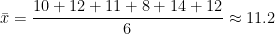
Find the mean of the data set below.
10
12
11
8
14
12
Using the idea above:
So, the mean for this data set is approximately 11.2. Looking at the original data, this does a good job of describing the center of this data set.
Calculation Using a TI83 or TI84 Graphing Calculator
The mean can easily be found using the function 1varstats on Ti83/84 graphing calculators. Here, we will go through the steps one by one. If you want to see a video of how to do this, scroll down to the bottom (or click here)!
Step 1: Enter your data in L1
To enter data in your calculator, press [STAT] and then go to 1: Edit by pressing [ENTER] or [1].
Now to enter the data, type each number and press enter. Note that if you already have data in your list, highlight the very top where it says L1 and press [CLEAR] followed by [ENTER].
Step 2: Calculate 1-var-stats
Once your data is in the list, press [STAT] again and then go to the CALC menu. From here, choose 1: 1varstats.
Now press enter twice and you will get a list of summary statistics. The first value that comes up is the mean!
Note: if you have a newer calculator, the menu looks a little different now. Instead of pressing enter twice, you will press enter and then have a 1-var stats menu come up. Just click CALCULATE at this menu and you will have the same information come up as you see above.
As you can see we get the exact same value as we did above. This is very nice for working with larger data sets.
As you will see below, dotplots are some of the easiest to read plots in statistics. That is, they are easy to read if you keep one thing in mind: each data value gets a dot and dots are stacked*. Of course, if you just came from our article on how to make dotplots, then you already know that. To understand how to read a dotplot, we will look at an example data set and see what kinds of questions we can answer.
[adsenseWide]
Answering questions from a dotplot
The dotplot below represents the fuel economy (in miles per gallon) for a sample of 2015 model year cars.
Use this dotplot to answer the following questions.
(a) How many vehicles are represented in the sample?
(b) What was the smallest value in the data set?
(c) How many vehicles in the sample get 31 mpg?
(d) What is the median mpg for vehicles in this sample?
This looks like a lot – let’s try each one individually.
(a) How many vehicles are represented in the sample?
Remembering our rule (each dot is a single data value), we can just count the number of dots. If you do that, you will find that there are 16. Therefore, we have 16 vehicles represented in the sample.
(b) What was the smallest value in the data set?
The horizontal scale represents the fuel economy, which are the values that make up our data set. The dot that represents the smallest value is just above the 16. So, 16 mpg is the smallest value in our data set. Phew – wouldn’t want to be filling up the tank for that car!
(if you are curious, that is the fuel economy for an Aston Martin V8 Vantage S – perhaps if that is the car you are driving, you aren’t too worried about fuel economy after all?)
(c) How many vehicles in the sample get 31 mpg?
The scale used here counts by 2; starting at 16. So, dots representing 31 are in between dots representing 30 and 32 on the scale. Counting these, there are 6 total dots. So, 6 of the sampled vehicles get 31 mpg.
(d) What is the median mpg for vehicles in this sample?
The median represent the middle value of a data set when it is placed in order from smallest to largest. If there are an even number of data values, like we have here (remember there are a total of 16 vehicles represented), then it is the average of the two middle values. For a data set with 16 values, this would be the average of the 8th and 9th value.
If you count from left to right (since the values have to be in order to find the median), the 8th and 9th values are both 31.
So, the median is \(\dfrac{31+31}{2}=31\) mpg.
You could also do this by listing out each of the values and then finding the average of the middle two. However, the more values there are, the more difficult this will be.
[adsenseLargeRectangle]
Summary
Dotplots are great at summarizing smaller data sets and they can be created by a large number of software programs. With most dotplots (see note before), you can identify each individual data value and use this information to understand the data set. This isn’t the case for other statistical plots, like histograms.
Notes:
*Some software programs will take large data sets and make it so that some dots represent 2 or more data values. This is always noted somewhere on the plot, so be on the lookout for it. You won’t usually come across this in an intro stats course, however.
Like histograms, dotplots are used to understand the pattern underlying a data set. Are most of the values large? Are most small? Unlike a histogram, the dotplot also shows you information about individual data values. So while a histogram can’t be used to answer the question “how many data values were 10?”, a dotplot can!
[adsenseWide]
So, let’s use an example to see how to make a nice dotplot. Note that many technology tools like Minitab can be used to create dotplots, but you may find in your typical statistics course you are making them by hand. Further, making a plot by hand is always a great way to get better at reading them.
Sketching a dotplot
The following data set shows the fuel economy (in miles per gallon) for a sample of 2015 model year vehicles.
Vehicle
Fuel Economy
Vehicle
Fuel Economy
Vehicle
Fuel Economy
Vehicle
Fuel Economy
Aston Martin V8 Vantage S
16
Hyundai Elantra
32
Kia Forte
31
Honda Accord
31
BMW 528i
27
Chevrolet Cruze
30
Buick Regal
24
Mazda 6
32
Subaru Legacy
30
Toyota Corolla
31
Lincoln MKZ Hybrid
40
Dodge Challenger
23
Dodge Dart
31
Lexus GS 450h
31
Subaru Impreza
31
Volvo V60 FWD
29
Now this data set definitely includes a wide variety of cars (although it is a bit of a small sample). It will be interesting to see the plot!
Step 1: Choose a scale and set it up.
We are going to make a horizontal scale and it needs to cover all values. For this data set, the smallest value is 16 and the largest is 40.
You will notice that I chose to count by 2 instead of 1. This isn’t required but just makes the plot a little more compact. You can count by 1, 5, or even 10 if you like!
Step 2: Plot the dots.
Alright, this step sounds goofy but there is really no other way to say it. For this step, you will start filling in the dots using your scale. Remember: Each value gets a dot and dots are “stacked”. To see this, let’s start by plotting only the first row of data.
Vehicle
Fuel Economy
Vehicle
Fuel Economy
Vehicle
Fuel Economy
Vehicle
Fuel Economy
Aston Martin V8 Vantage S
16
Hyundai Elantra
32
Kia Forte
31
Honda Accord
31
You can see that each value is represented by a dot on the plot and that, since there were two cars that get 31 mpg, we put two dots on top of each other. Now we can continue the process with the rest of the data. Remember that while you can’t be perfect doing this by hand, that you should try and make sure that the dots mostly line up. You don’t want any big spaces between dots to make one value look more common than another.
Here is the data set along with the finished dotplot. You can see again, each value got a dot. Notice that we added a title and a label to our main scale. This step is important so someone else looking at the plot can know what kind of data they are looking at.
Vehicle
Fuel Economy
Vehicle
Fuel Economy
Vehicle
Fuel Economy
Vehicle
Fuel Economy
Aston Martin V8 Vantage S
16
Hyundai Elantra
32
Kia Forte
31
Honda Accord
31
BMW 528i
27
Chevrolet Cruze
30
Buick Regal
24
Mazda 6
32
Subaru Legacy
30
Toyota Corolla
31
Lincoln MKZ Hybrid
40
Dodge Challenger
23
Dodge Dart
31
Lexus GS 450h
31
Subaru Impreza
31
Volvo V60 FWD
29
That really is it! The dotplot is a great plot to use for representing data precisely because it is so simple to make and read. Remember that in statistics, our goal is often to communicate information to others. The more simply we can do this, the better.
For some examples of the types of questions you might run across when it comes to dotplots and what information you can gather from them, check out “How to read a dotplot” next.
The logic of hypothesis testing can be really confusing. Why do we “reject ” or “fail to reject “, and what does that really mean? Did we prove the null hypothesis when we didn’t reject it? These are common questions for any student studying these ideas.
It turns out that we have a very nice example of the logic behind hypothesis testing right in your everyday NFL or college football game. The basic idea comes from the “challenge” that a coach can use to dispute a call on the field by a referee. For example, a referee may say that the other team has scored. But, it is a very close play and the other team thinks that the referee could be wrong. At this point, the coach of that team may elect (under certain conditions) to challenge the call. Once a call is challenged, the play call is reviewed. During the review, the referees are looking for “clear evidence” that the play on the field was incorrect. If they find it, they will overturn the call. If not, they will make the statement “the ruling on the field stands” and that’s that. The game continues.
The sentence that should catch the eye of any statistics student is the phrase “the ruling on the field stands”. The ref’s are very careful not to say “the ruling on the field was correct” – instead, they elect to say something that implies “we didn’t see enough evidence to overturn the call”. These are two very different things! It is sort of like a court of law. We don’t find people innocent; instead, we find them “not guilty”. In other words, we didn’t see any evidence to change our minds from the assumption that they were innocent.
The Null Hypothesis
In hypothesis testing, the null hypothesis () is assumed to be true. So, to test a claim about the population, we take a sample and then we then look at the “evidence” (a p-value or a test statistic) to determine if the sample we took is unique enough to make us reject our assumption. That is, we decide to reject the null hypothesis or fail to reject the null hypothesis. We only do this if there is significant evidence , in other words, a “small” p-value (p-value smaller than ).
In the football example, the null hypothesis would be “the call on the field is correct” and the evidence would be the video replays available to the referees. The null hypothesis will only be rejected if there is significant evidence to the contrary.
Now, here is the tricky part. We can never PROVE the null hypothesis is true because we base all of our calculations on assuming it is true. We can only state whether there is evidence against it. Of course, in our football example , the referees probably could actually prove that the original call was correct, but reviewed plays are often a bit borderline (and I’m sure no one wants to say “that other ref was wrong”) so they choose to simply state that there is evidence against the null hypothesis. That is, that there is enough video evidence to make them change their minds about the call. This is the same as saying “we reject the null hypothesis”.
The Alternative Hypothesis
The competing hypothesis is the alternative (). We can almost think of this as the hypothesis that “something interesting is happening”. In other words, whatever we want to prove – whether it be that sales are increased by talking to customers or that a certain medicine reduces the number of headaches – will be the alternative hypothesis. When we reject (), we are saying there is evidence towards the alternative hypothesis. We are saying that the sample is unique enough under the null hypothesis to make us question it altogether.
When the refs overturn a call, they are saying “we reject (), there is evidence towards the alternative hypothesis”. That is, “we have enough evidence to make us question the original call”. In this case, the video was enough to make them seriously question the null hypothesis (that the call was correct).
Failing to Reject the Null
Thinking about all of this, failing to reject doesn’t say much. In the case of our friends the NFL ref’s, it simply means that there wasn’t enough evidence to make them change their minds about the call being correct. They aren’t saying it was correct, just that they can’t , based on this evidence, overturn the call.
In an experiment where we are trying to prove that a headache medicine reduces the average number of headaches patients experience each week, failing to reject would mean that there is no evidence that the medicine does in fact reduce this number. Any changes in the number of headaches experienced by patients could be due to chance. It doesn’t mean that the medicine absolutely doesn’t work. It just means that our study doesn’t prove that it does.
Practical Considerations
Suppose we were really trying to prove some headache medicine worked and in the end, we failed to reject our null hypothesis. What then?
Of course, we didn’t prove , so it may be that our medicine works (but effects are LIKELY due to chance since we didn’t reject the null). But since we didn’t prove that it does, the FDA will never let us sell it to consumers. So even though we didn’t prove the null hypothesis, real life dictates that there are consequences to not rejecting it that are very similar to having proved it.
Similarly, suppose that I run a factory and you try to sell me a system that reduces errors (supposedly). I run a test and find that I can’t prove it does in fact reduce errors ( I fail to reject ). Do I say “well, you can’t PROVE , so I will buy the system”? No, I will likely make the decision as though is true and therefore not buy it because it wasn’t proven to work. This is just practicality. My decision is based on the fact that you didn’t prove the alternative, .
As you study hypothesis testing (z-tests, t-tests, and others), you may find some of the language and required statements a bit rigid and maybe almost lawyer-like. Now you can see that a lot of this comes from us trying to work about ideas of uncertainty and what you can and cannot prove. We have to be careful and make sure that we don’t say things like “ is true” or even “ is true” because in the end we are working with probabilities and assumptions. The only time we could really say these things is if we could work with the entire population (and then we wouldn’t even need hypothesis testing – think about that one!).
In order to estimate the value of an unknown population mean, we can use a confidence interval based on the standard normal distribution (z-interval) or the t-distribution (t-interval). The choice is usually determined by the following rule:
Use a z-interval if: the population standard deviation is known and either the population is normally distributed or the sample size is larger than 30.
Use a t-interval if: the population standard deviation is unknown and either the population is normally distributed or the sample size is larger than 30.
[adsenseWide]
In both cases, you can either use the formula to compute the interval by hand or use a graphing calculator (or other software). In this article, we will see how to use the TI83/84 calculator to calculate z and t intervals. Note: You can scroll down to see a video of these steps!
z-Intervals
A psychologist wants to estimate the amount of time college students spend browsing the internet each day. In a sample of 32 college students, the average time spent browsing the internet each day was about 67 minutes. If it is believed that the population standard deviation is 14 minutes, then calculate a 95% confidence interval to estimate the average time spent by college students browsing the internet each day.
In this example, we are told that the population standard deviation is thought to be 14 minutes and we have a large enough sample size. Therefore, a z-interval can be used to calculate the confidence interval.
Step 1: Go to the z-interval on the calculator.
Press [STAT]->Calc->7. Z-interval [ENTER]
Step 2: Highlight STATS
Since we have statistics for the sample already calculated, we will highlight STATS at the top. If you had a list of data instead, you could enter it into L1 and then use DATA. This is really only useful for small data sets.
Step 3: Enter Data
Notice that the calculator asks for sigma (the population standard deviation) – this should help you remember that you shouldn’t be using this unless you have sigma already.
Step 4: Calculate and interpret
Please make sure to read the explanation of how to interpret intervals in general. It is very easy to misunderstand what they truly mean! Highlight CALCULATE and then press ENTER to get your interval.
Here we are given our 95% confidence interval as (62.149, 71.851). This means that we are 95% confident that the true mean time that college students spend browsing the internet each day is between 62.15 minutes and 71.85 minutes. Note – there are many other ways to write this interval.
t-intervals
When the population standard deviation is unknown, we will use a t-interval to estimate the mean. Using a t-interval on the calculator has almost the same steps as using a z-interval, as you will see below.
For a statistics project, a student samples 37 high school teachers in her community and records how many years they have worked in education. In her sample, the average number of years was 14.2 with a standard deviation of 6.8. Use this information to estimate the mean number of years worked in education for all high school teachers in the community by calculating a 99% confidence interval.
Notice that in this example, the standard deviation is coming from the sample. Therefore, this is not sigma (the population standard deviation) but instead s (the sample standard deviation). This means we should use a t-interval for this estimate.
Step 1: Go to the t-interval on the calculator.
Press [STAT]->Calc->8. t-interval then [ENTER].
Step 2: Highlight STATS
Since we have statistics for the sample already calculated, we will highlight STATS at the top. If you had a list of data instead, you could enter it into L1 and then use DATA. This is really only useful for small data sets.
Step 3: Enter Data
Notice this time that the calculator asks for s – the sample standard deviation.
Step 4: Calculate and interpret
All you have to do is highlight CALCULATE and press ENTER.
So our 99% confidence interval is (11.16, 17.24). We can interpret this by saying “We are 99% confident that the mean number of years spent working in education by high school teachers in this community is between 11.16 years and 17.24 years.”
[adsenseLargeRectangle]
Video walkthrough
The following video will walk you through the steps for a t-interval or z-interval on the TI83/84 calculator.
Before you ever even thought about statistics, you had seen a confidence interval for a proportion. Don’t believe me? Well think back – does this sound familiar?
“A new poll shows that 45% of Americans believe something interesting about some idea….(on the screen is a note: *margin of error 4%)”
Yup, that exciting piece of news (I really should be a news writer come to think of it) is really representing a confidence interval for some population proportion. We use these types of confidence intervals anytime we want to understand the percentage or proportion of a population that has a certain property. The idea is to take a sample, see what percentage of our sample has the property, and finally use these calculations to estimate how well that translates to the whole group or population.
[adsenseWide]
Important symbols:
P-hat or is the sample proportion. It can be found by dividing the sample number of successes x (whatever we are counting) by the sample size n
p will represent the population proportion. In some textbooks, is used
The Assumptions
In order to use these procedures, we will need to have the central limit theorem for sample proportions (the big ideas of this theorem are for another article and day). This means that it’s initial assumptions must hold. Those are:
We have a random sample from the population.
The population size is much larger than the sample size
We have a “big enough” sample. In this case we will need AND
For these examples, we will assume that the first two statements are true, but we will check the last condition. Remember that if you are working with real data in a research situation, that you must be careful to make sure the first two conditions holds as well.
The Calculation – By Hand
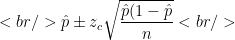
The general formula for this type of confidence interval is:
where is a critical value from the normal distribution (see below) and is the sample size.
Common values of are:
Confidence Level
Critical Value
90%
1.645
95%
1.96
99%
2.575
Now that we have that out of the way, let’s try it on an example!
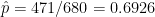
In a sample of 680 young adults (ages 18 – 25) residing in a large city, 471 stated that they regularly use public transportation. Use this information to calculate a 95% confidence interval for the proportion of all young adults in this city that regularly use public transportation.
Since we are estimating a population proportion, we know that we will use the formula above. Before we can use that formula though, we must check assumptions. Here and while . Both of these numbers are larger than 10 so we can continue.
The formula:
Plugging values in:
Simplifying:
Note that in the last step, I did every calculation in my calculator and avoided rounding until the end. To see this “in action” Please check the video of this example on the right hand side of your screen. At this stage, you can convert to percentages and use this as your final answer.
With all confidence intervals, it is easy to get caught up in the calculations and forget that they have a real world meaning. Not only that, but the real world meaning is often confused or misunderstood. Make sure you read about how to interpret confidence intervals and take note of the common misinterpretations.
In this example, we could say We are 95% confidence that between 66% and 72% of all young adults in this city regularly use public transportation. This means that about 95% of the time, an interval produced this way will work as intended. In other words, about 95% of the time, the actual percentage will be between the two values we calculate. (still confused? Read the article linked above!)
Assuming that you are familiar with how to calculate a confidence interval as well as how to interpret a confidence interval, you may be curious as to actually write down a final “answer” or result. The following lesson will show you some different ways that confidence intervals can be written.
[adsenseWide]
Example
We will use the following example to think about the different ways to write a confidence interval. For practice, you should make sure you know how to do the calculations needed to get the interval.
A college student wishes to estimate the percentage of students on his campus who can name the current president of the college. He chooses a random sample of 347 students and finds that 86 of them can in fact, name the current college president. Help the student estimate the percentage of all students who can name the current president by calculating a 95% confidence interval.
Let’s think about different ways this interval might be written.
Method 1 – point estimate +/- margin of error
All confidence intervals are of the form “point estimate” plus/minus the “margin of error”. If you are finding a confidence interval by hand using a formula (like above), your interval is in this form before you do your addition or subtraction. This is a common way to actually present your confidence interval.
Final Answer: \(0.248 \pm 0.045\)
Since this confidence interval is estimating a percentage, it might also be written as:
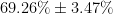
Final Answer: \(24.8\% \pm 4.5\%\)
This would be the method probably used on the news or in any report to a general audience. The student could say “about 24.8% of students at my college can name the college president.” He would then also note that his estimate has a margin of error of 4.5%. If you pay attention to the evning news or new articles, they typically show this number on the screen or mention it in the article while discussing similar polls.
Method 2 – as an interval
If you actually do the two calculations, 0.248 – 0.045 = 0.203 and 0.248 + 0.045 = 0.293, you will get two endpoints. These can be used to write the final answer as well.
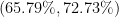
Final Answer: \((0.203, 0.293)\)
Or, if using percentages:
Final Answer: \((20.3\%, 29.3\%)\)
This is typically how a confidence interval will look if you calculating it using technology such as a ti83 or ti84. It’s a little more “mathy” so you might not see it as often in reports to general audiences.
Method 3 – as an inequality
Finally, some textbooks like to write intervals in a way to help you remember that somewhere in that interval is your population value you are trying to estimate. In this case, you are estimating the population proportion p, so you would write.
Final Answer: \(0.203 < p < 0.293\)
Note that if you were estimating the mean, you would place \(\mu\) within the inequality.
[adsenseLargeRectangle]
Important
If you are taking a statistics course, it is of important to pay attention to how your professor or textbook prefers to present confidence intervals and generally stick to that method. If instead, you are using confidence intervals in your research, it is probably important to consider your audience. Most people have no trouble understanding the idea of adding and subtracting a margin of error, even if they haven’t had much formal training in statistics. This should be a consideration when you present your findings.
Finally, and most importantly, do take a moment to read about how to interpret confidence intervals. It is easy to get caught up in the math side but you still must know how this applies to real life situations.
When dealing with any type of probability question, the sample space represents the set or collection of all possible outcomes. In other words, it is a list of every possible result when running the experiment just once. For example, in one roll of a die, a 1, 2, 3, 4, 5, or 6 could come up. Each of these are considered outcomes and together they make up a sample space. In the following lesson, we will look at the notation used for a sample space as well as some examples of finding the sample space for a probability experiment.
[adsenseWide]
Notation
Sample spaces are usually written using set notation. This means that each possibility is listed only once within curly brackets. For example, if there were three possibilities we would write the sample space as:
Many times, the outcomes will be written in some kind of shorthand. It is not necessary to use shorthand when writing out the possibilities, but if you do, make sure that the shorthand is easy to follow. For example, suppose we flipped a coin. The possibilities are “heads” and “tails” which could be written as “H” and “T”. Using this, the sample space would be:
\(S = \{ \text{H}, \text{T} \}\)
Examples of finding the sample space
With any type of probability experiment, describing the sample space just requires thinking carefully about all of the possibilities and making sure none are missed. You can see this type of thinking in the examples below.
Example
A single 12 sided die has the whole numbers 1 through 12 written on each face. The die is rolled once and the number that appears is noted. Describe the sample space of this experiment.
Solution
Any of the 12 sides could have come up on a single roll. Therefore the sample space would be
Suppose that two coins are flipped and the side which they land on is noted. Describe the sample space for this experiment.
Solution
One possibility is that both coins land on the same side. If this was the case, that side could be either heads or tails. These two outcomes could be represented by HH and TT. If the coins don’t land on the same sides then what are the other possibilities? Well, it could be the first coin landed on heads and the second tails (HT) or the other way around (TH). Notice that when we deal with sample spaces, the order is important!
\(S = \left\{ HH, TT, HT, TH \right\}\)
Example
A person is asked to guess a random number between 1 and 10 and it is noted whether or not he guessed correctly. Describe the sample space for this experiment.
Solution
This one is much trickier than it looks! Notice that the number being guessed doesn’t matter here – all that is being noted is if the number was guessed correctly (possibility 1) or if the number was not guessed correctly (possibility 2). There is nothing in between him guessing right or wrong, so this covers all of our possibilities!
This last example shows how important the context is. If we were interested in the possible numbers he could have guessed, then our sample space would have looked completely different. Paying attention to details like this is important in all probability calculations.
[adsenseLargeRectangle]
Summary
The sample space of an experiment is just a listing of all the possible outcomes (results) from that experiment. To find the sample space, you need to make sure you think of all the possible results. Be sure to pay close attention to the context and what aspect of the probability experiment is of interest.
A confidence interval is a way of using a sample to estimate an unknown population value. For estimating the mean, there are two types of confidence intervals that can be used: z-intervals and t-intervals. In the following lesson, we will look at how to use the formula for each of these types of intervals. To see the examples below in a video, scroll down!
This procedure is often used in textbooks as an introduction to the idea of confidence intervals, but is not really used in actual estimation in the real world. Even so, it is common enough that we will talk about it here!
What makes it strange? Well, in order to use a z-interval, we assume that \(\sigma\) (the population standard deviation) is known. As you can imagine, if we don’t know the population mean (that’s what we are trying to estimate), then how would we know the population standard deviation?
When to use a z-interval
Setting the discussion above aside, the general rule for when to use a z-interval calculation is:
Use a z-interval when:
the sample size is greater than or equal to 30 and population standard deviation known OR Original population normal with the population standard deviation known.
Formula for the z-interval
If these conditions hold, we will use this formula for calculating the confidence interval:
where \(z_{c}\) is a critical value from the normal distribution (see below) and \(n\) is the sample size.
Common values of \(z_{c}\) are:
Confidence Level
Critical Value
90%
1.645
95%
1.96
99%
2.575
Example using a z-interval
Suppose that in a sample of 50 college students in Illinois, the mean credit card debt was $346. Suppose that we also have reason to believe (from previous studies) that the population standard deviation of credit card debts for this group is $108. Use this information to calculate a 95% confidence interval for the mean credit card debt of all college students in Illinois.
Solution
Since we wish to estimate the mean, we immediately know we will be using either a t-interval or a z-interval. Looking a bit closer, we see that we have a large sample size (\(n = 50\)) and we know the population standard deviation. Therefore, we will use a z-interval with \(z_{c} = 1.96\). From reading the problem, we also have:
This gives our 95% confidence interval for \(\mu\), the population mean, as \(\boxed{(316.1, 375.9)}\).
Interpretation
We are 95% confident that the mean amount of credit card debt for all college students in Illinois is between $316.10 and $375.90.
Of course this is a very particular statement, so please make sure you study how to interpret confidence intervals in general and so you can understand exactly what this means.
Other ways to write this interval
Another way to present this interval would be to calculate the margin of error:
\(1.96\left(\dfrac{108}{50}\right)=29.9\)
and write the interval as:
\(\boxed{$346} \pm \$29.9\)}
Both versions are correct, and the version you use depends on your audience and perhaps your teacher or professors preference. You can read more about different ways to write intervals here: Three ways to write a confidence interval.
T-intervals
The much more realistic scenario is using a t-interval to estimate an unknown population mean. This interval relies on our sample standard deviation in calculating the margin of error. All this means for us is that the formula will be very similar, but the critical value will no longer come from the normal distribution. Instead, it will come from the student’s t distribution.
When to use a t-interval
The rules for when to use a t-interval are as follows.
Use a t-interval when:
Population standard deviation UNKNOWN and original population normal OR sample size greater than or equal to 30 and Population standard deviation UNKNOWN.
where \(t_{c}\) is a critical value from the t-distribution, \(s\) is the sample standard deviation and \(n\) is the sample size.
Finding \(t_c\)
The value of \(t_{c}\) depends on the sample size through the use of “degrees of freedom” where \(df = n – 1\). We will use this to look up the value of \(t_{c}\) in a table (a nice free version of that table can be found here, or typically in the back of your textbook if you are currently taking a class).
Example using a t-interval
Suppose that a sample of 38 employees at a large company were surveyed and asked how many hours a week they thought the company wasted on unnecessary meetings. The mean number of hours these employees stated was 12.4 with a standard deviation of 5.1. Calculate a 99% confidence interval to estimate the mean amount of time all employees at this company believe is wasted on unnecessary meetings each week.
Solution
As before, since we are estimating a mean with a confidence interval, we know it will either be a t-interval or a z-interval. In this case, we have a large sample (\(n = 38\)), but we only have the sample standard deviation. If you aren’t sure of that – read closely. The standard deviation of 5.1 was in the context of the sample, so \(s = 5.1\). Thus, we will go ahead and use a t-interval since \(\sigma\) is unknown.
Before we can do that however, we need to look up the critical value. To know which row in the t-table to look at, we find the degrees of freedom which is \(n – 1 = 38 – 1 = 37\). Using the table linked here:
Now that we have that, we plug the values into the formula and do the calculations to get our two endpoints. Remember that we have:
99% Confidence Interval for \(\mu\): \(\boxed{(10.2, 14.6)}\)
Interpretation
“We are 99% confident that the mean amount of time that all employees at this company think is wasted on meetings each week is between 10.2 and 14.6 hours.”
The same warning applies here – make sure you take the time to truly study what this means.
Video of the examples
The following video goes through the examples completed above. Use this to help yourself better understand how to apply these formulas.
Other Considerations
Confidence intervals are most often calculated with tools like SAS, SPSS, R, (these are statistical calculations packages) Excel, or even a graphing calculator. It is helpful to calculate them by hand once or twice to get a feel for the concept but you should also take the time to learn how to calculate them using one of these common tools. Which tool you use depends on the course you are taking or the field you are working in.
[adsenseLargeRectangle]
Additional Reading
If you are currently taking a statistics course, we have a ton of free statistics lessons and videos. Be sure to check out the statistics section on MathBootCamps for more articles like this one!
The general idea of any confidence interval is that we have an unknown value in the population and we want to get a good estimate of its value. Using the theory associated with sampling distributions and the empirical rule, we are able to come up with a range of possible values, and this is what we call a “confidence interval”.
[adsenseWide]
When interpreting the meaning, the key phrase to understand is “confidence”. If I am 95% confident the true mean is before 4 and 10, what am I actually saying?
Thinking About the Meaning of “95% Confident”
Let’s use an example to understand some possible interpretations in context. Suppose that we have a good (the sample was found using good techniques) sample of 45 people who work in a particular city. It took people in our sample an average time of 21 minutes to get to work one -way. The standard deviation was 9 minutes.
Calculating a 95% confidence interval for the mean using a t-interval for the population mean, we get : (18.3, 23.7). To start understanding the interval, we will look at some common misconceptions:
FALSE INTERPRETATION: “95% of the 45 workers take between 18.3 and 23.7 minutes to get to work”.
While we used a sample to get the estimate, we are no longer talking about the sample. The confidence interval is now about ALL the workers that work in the city, not just the 45.
FALSE INTERPRETATION: “There is a 95% chance that the mean time it takes all workers in this city to get to work is between 18.3 and 23.7 minutes”.
This is a very common misconception! It seems very close to true, but it isn’t because the population mean value is fixed. So, it is either in the interval or not. This is subtle but important.
What is correct?
95% of the time, when we calculate a confidence interval in this way, the true mean will be between the two values. 5% of the time, it will not. Because the true mean (population mean) is an unknown value, we don’t know if we are in the 5% or the 95%. BUT 95% is pretty good so we say something like
“We are 95% confident that the mean time it takes all workers in this city to get to work is between 18.3 and 23.7 minutes.” This is a common shorthand for the idea that the calculations “work” 95% of the time.
Remember that we can’t have a 100% confidence interval. By definition, the population mean is not known . If we could calculate it exactly we would! But that would mean that we need a census of our population with is often not possible or feasible.
Why Don’t We Always Use a 99% Confidence Level?
Seems to make sense right? Get the confidence level as high as you can! Well, as the confidence level increases, the margin of error increases . That means the interval is wider. So, it may be that the interval is so large it is useless! For example, what if I said that I am 99% confident that you will score between a 10 and a 100 on your next exam? How useful is that in predicting your performance? The interval is simply too wide. There are some instances where it doesn’t matter as much, but that is on a case by case basis.
For this reason, 95% confidence intervals are the most common. You will sometimes see 80% or others in textbooks, but in real applications it’s almost always a 95% interval with occasional 90% and 99% intervals being used.
CI for Parameters Other than the Mean
Confidence intervals can be calculated for many other population parameters and the interpretation still remains generally the same. Using the shorthand “we are 95% confident that…”, we will state that we are “pretty sure” that the parameter (the mean, the population proportion, etc) is within the given range.
As an example, suppose we have a 99% confidence interval of (0.122, 0.141) for the proportion of likely voters that approve a new measure. Then we could say:
“We are 99% confident that the proportion of all likely voters that approve the new measure is between 0.122 and 0.141”
Better yet, we could say:
“We are 99% confident that the percentage of all likely voters that approve the new measure is between 12.2% and 14.1%”
This is easier to explain to someone who hasn’t had statistics. In fact, anytime you see a poll on the news with a margin of error, they are likely talking about a confidence interval! They just tend to give the point estimate and the margin of error instead of the whole interval.
For example, when they say “a poll found 52% of people approve of the president” and you see on the screen “margin of error: 2%” then you know they are talking about a confidence interval of (50%, 54%). (they tend not to give the confidence level as that is a bit technical for a general news broadcast).


 ” or “fail to reject
  ).
).
 ). We can almost think of this as the hypothesis that “something interesting is happening”. In other words, whatever we want to prove – whether it be that sales are increased by talking to customers or that a certain medicine reduces the number of headaches – will be the alternative hypothesis. When we reject (


 So our 99% confidence interval is (11.16, 17.24). We can interpret this by saying “We are 99% confident that the mean number of years spent working in education by high school teachers in this community is between 11.16 years and 17.24 years.”
 is the sample proportion. It can be found by dividing the sample number of successes x (whatever we are counting) by the sample size n
 is used
 AND
AND 
 is a critical value from the normal distribution (see below) and
  is the sample size.
 and
and  while
while  . Both of these numbers are larger than 10 so we can continue.