The idea of a linear combination of vectors is very important to the study of linear algebra. We can use linear combinations to understand spanning sets, the column space of a matrix, and a large number of other topics. One of the most useful skills when working with linear combinations is determining when one vector is a linear combination of a given set of vectors.
[adsenseWide]
Suppose that we have a vector \(\vec{v}\) and we want to know the answer to the question “is \(\vec{v}\) a linear combination of the vectors \(\vec{a}_{1}\), \(\vec{a}_{2}\), and \(\vec{a}_{3}\)?”. Using the definition of a linear combination of vectors, this question can be restated to the following:
Are there scalars \(x_{1}\), \(x_{2}\), and \(x_{3}\) such that:
\(\vec{v} = x_1\vec{a}_{1 }+x_2\vec{a}_{2}+ x_3\vec{a}_{3}\)?
If the vectors are in \(R^n\) for some \(n\), then this is a question that can be answered using the equivalent augmented matrix:
\(\left[ \begin{array}{ccc|c} \vec{a}_1 & \vec{a}_2 & \vec{a}_3 & \vec{v} \\ \end{array} \right]\)
If this matrix represents a consistent system of equations, then we can say that \(\vec{v}\) is a linear combination of the other vectors.
Example
Determine if the vector \(\begin{bmatrix} 5 \\ 3 \\ 0 \\ \end{bmatrix}\) is a linear combination of the vectors:
\(\begin{bmatrix} 2 \\ 0 \\ 1 \\ \end{bmatrix}\), \(\begin{bmatrix} 1 \\ 4 \\ 3 \\ \end{bmatrix}\), \(\begin{bmatrix} 8 \\ 1 \\ 1 \\ \end{bmatrix}\), and \(\begin{bmatrix} -4 \\ 6 \\ 1 \\ \end{bmatrix}\)
Solution
Remember that this means we want to find constants \(x_{1}\), \(x_{2}\), \(x_{3}\), and \(x_{4}\) such that:
\(\begin{bmatrix} 5 \\ 3 \\ 0 \\ \end{bmatrix} = x_{1}\begin{bmatrix} 2 \\ 0 \\ 1 \\ \end{bmatrix} + x_{2}\begin{bmatrix} 1 \\ 4 \\ 3 \\ \end{bmatrix} + x_{3}\begin{bmatrix} 8 \\ 1 \\ 1 \\ \end{bmatrix} + x_{4}\begin{bmatrix} -4 \\ 6 \\ 1 \\ \end{bmatrix}\)
This vector equation is equivalent to an augmented matrix. Setting this matrix up and row reducing, we find that:
\(\left[ \begin{array}{cccc|c} 2 & 1 & 8 & -4 & 5 \\
0 & 4 & 1 & 6 & 3 \\
1 & 3 & 1 & 1 & 0 \\
\end{array} \right]
\)
Is equivalent to:
\(\left[ \begin{array}{cccc|c} 1 & 0 & 0 & -\frac{103}{29} & -\frac{74}{29} \\
0 & 1 & 0 & \frac{42}{29} & \frac{13}{29} \\
0 & 0 & 1 & \frac{6}{29} & \frac{35}{29} \\
\end{array}\right]\)
While it isn’t pretty, this matrix does NOT contain a row such as \(\begin{bmatrix} 0 & 0 & 0 & 0 & c \\ \end{bmatrix}\) where \(c \neq 0\) which would indicate the underlying system is inconsistent. Therefore the underlying system is consistent (has a solution) which means the vector equation is also consistent.
So, we can say that \(\begin{bmatrix} 5 \\ 3 \\ 0 \\ \end{bmatrix}\) is a linear combination of the other vectors.
The step-by-step process
In general, if you want to determine if a vector \(\vec{u}\) is a linear combination of vectors \(\vec{v}_{1}\), \(\vec{v}_{2}\), … , \(\vec{v}_{p}\) (for any whole number \(p > 2\)) you will do the following.
Step 1
Set up the augmented matrix
\(\left[ \begin{array}{cccc|c} \vec{v}_1 & \vec{v}_2 & \cdots & \vec{v}_p & \vec{u} \\ \end{array} \right]\)
and row reduce it.
Step 2
Use the reduced form of the matrix to determine if the augmented matrix represents a consistent system of equations. If so, then \(\vec{u}\) is a linear combination of the others. Otherwise, it is not.
In the second step, it is important to remember that a system of equations is consistent if there is one solution OR many solutions. The number of solutions is not important – only that there IS at least one solution. That means there is at least one way to write the given vector as a linear combination of the others.
Writing a Vector as a Linear Combination of Other Vectors
Sometimes you might be asked to write a vector as a linear combination of other vectors. This requires the same work as above with one more step. You need to use a solution to the vector equation to write out how the vectors are combined to make the new vector.
Let’s start with an easier case than the one we did before and then come back to it since it is a bit complicated.
Example
Write the vector \(\vec{v} = \begin{bmatrix} 2 \\ 4 \\ 2 \\ \end{bmatrix}\) as a linear combination of the vectors:
\(\begin{bmatrix} 2 \\ 0 \\ 1 \\ \end{bmatrix}\), \(\begin{bmatrix} 0 \\ 1 \\ 0 \\ \end{bmatrix}\), and \(\begin{bmatrix} -2 \\ 0 \\ 0 \\ \end{bmatrix}\)
Solution
Step 1
We set up our augmented matrix and row reduce it.
\(
\left[ \begin{array}{ccc|c} 2 & 0 & -2 & 2 \\
0 & 1 & 0 & 4 \\
1 & 0 & 0 & 2 \\
\end{array} \right]
\)
is equivalent to
\(
\left[ \begin{array}{ccc|c} 1 & 0 & 0 & 2 \\
0 & 1 & 0 & 4 \\
0 & 0 & 1 & 1 \\
\end{array} \right]
\)
Step 2
We determine if the matrix represents a consistent system of equations.
Based on the reduced matrix, the underlying system is consistent. Again, this is because there are no rows of all zeros in the coefficient part of the matrix and a single nonzero value in the augment. (you could also use the number of pivots to make the argument.)
Unlike before, we don’t only want to verify that we have a linear combination. We want to show the linear combination itself. This means that we need an actual solution. In this case, there is only one:
\(x_1 = 2\), \(x_2 = 4\), \(x_3 = 1\)
Using these values, we can write \(\vec{v}\) as:
\(\vec{v} = \begin{bmatrix} 2 \\ 4 \\ 2 \\ \end{bmatrix} = (2)\begin{bmatrix} 2 \\ 0 \\ 1 \\ \end{bmatrix} + (4)\begin{bmatrix} 0 \\ 1 \\ 0 \\ \end{bmatrix} + (1)\begin{bmatrix} -2 \\ 0 \\ 0 \\ \end{bmatrix}\)
Now let’s go back to our first example (the one with the crazy fractions) but change the instructions a bit.
Example
Write the vector \(\vec{v} = \begin{bmatrix} 5 \\ 3 \\ 0 \\ \end{bmatrix}\) as a linear combination of the vectors:
\(\begin{bmatrix} 2 \\ 0 \\ 1 \\ \end{bmatrix}\), \(\begin{bmatrix} 1 \\ 4 \\ 3 \\ \end{bmatrix}\), \(\begin{bmatrix} 8 \\ 1 \\ 1 \\ \end{bmatrix}\), and \(\begin{bmatrix} -4 \\ 6 \\ 1 \\ \end{bmatrix}\)
When we did step 1, we had the following work. This showed that the equivalent vector equation was consistent and verified that \(\vec{v}\) was a linear combination of the other vectors.
\(\left[ \begin{array}{cccc|c} 2 & 1 & 8 & -4 & 5 \\
0 & 4 & 1 & 6 & 3 \\
1 & 3 & 1 & 1 & 0 \\
\end{array} \right]
\)
Is equivalent to:
\(\left[ \begin{array}{cccc|c} 1 & 0 & 0 & -\frac{103}{29} & -\frac{74}{29} \\
0 & 1 & 0 & \frac{42}{29} & \frac{13}{29} \\
0 & 0 & 1 & \frac{6}{29} & \frac{35}{29} \\
\end{array}\right]\)
What if we wanted to write out the linear combination. This is different from the previous example in that there are infinitely many solutions to the vector equation.
Looking more closely at this augmented matrix, we can see that there is one free variable \(x_{4}\). If we write out the equations, we have:
\(x_1 – \left(\frac{103}{29}\right)x_4 = -\frac{74}{29}\)
\(x_2 + \left(\frac{42}{29}\right)x_4 = \frac{13}{29}\)
\(x_3 + \left(\frac{6}{29}\right)x_4 = \frac{35}{29}\)
Since \(x_{4}\) is a free variable, we can let it have any value and find a solution to this system of equations. A really “nice” value would be zero. If \(x_4 = 0\), then:
\(x_1 – \frac{103}{29}(0) = -\frac{74}{29}\)
\(x_2 + \frac{42}{29}(0) = \frac{13}{29}\)
\(x_3 + \frac{6}{29}(0) = \frac{35}{29}\)
Using this solution, we can write \(\vec{v}\) as a linear combination of the other vectors.
\(\vec{v} = \begin{bmatrix} 5 \\ 3 \\ 0 \\ \end{bmatrix} = \left(-\frac{72}{29}\right)\begin{bmatrix} 2 \\ 0 \\ 1 \\ \end{bmatrix} + \left(\frac{13}{29}\right)\begin{bmatrix} 1 \\ 4 \\ 3 \\ \end{bmatrix} + \left(\frac{35}{29}\right)\begin{bmatrix} 8 \\ 1 \\ 1 \\ \end{bmatrix} + (0)\begin{bmatrix} -4 \\ 6 \\ 1 \\ \end{bmatrix}\)
This would be one solution, but because \(x_4\) is free, there are infinitely many. For each possible value of \(x_4\), you have another correct way to write \(\vec{v}\) as a linear combination of the other vectors. For example, if \(x_4 = 1\):
\(\begin{align}x_1 &= -\frac{74}{29} + \frac{103}{29} \\ &= \frac{29}{29} \\ &= 1\end{align}\)
\(\begin{align}x_2 &= \frac{13}{29} – \frac{42}{29}\\ &= -\frac{29}{29} \\ &= -1\end{align}\)
\(\begin{align}x_3 &= \frac{35}{29} – \frac{6}{29}\\ &= \frac{29}{29} \\ &= 1\end{align}\)
Using this, we can also write:
\(\vec{v} = \begin{bmatrix} 5 \\ 3 \\ 0 \\ \end{bmatrix} = (1)\begin{bmatrix} 2 \\ 0 \\ 1 \\ \end{bmatrix} + (-1)\begin{bmatrix} 1 \\ 4 \\ 3 \\ \end{bmatrix} + (1)\begin{bmatrix} 8 \\ 1 \\ 1 \\ \end{bmatrix} + (1)\begin{bmatrix} -4 \\ 6 \\ 1 \\ \end{bmatrix}\)
How nice is that? (note: normally, we wouldn’t write out the 1 in the equation showing the linear combination. I left it there so you could see where each number from the solution ended up).
Again, a problem like this has infinitely many answers. All you have to do is pick a value for the free variables and you will have one particular solution you can use in writing the linear combination.
When the Vector is NOT a Linear Combination of the Others
It is worth seeing one example where a vector is not a linear combination of some given vectors. When this happens, we will end up with an augmented matrix indicating an inconsistent system of equations.
Example
Determine if the vector \(\begin{bmatrix} 1 \\ 2 \\ 1 \\ \end{bmatrix}\) is a linear combination of the vectors:
\(\begin{bmatrix} 1 \\ 1 \\ 0 \\ \end{bmatrix}\), \(\begin{bmatrix} 0 \\ 1 \\ -1 \\ \end{bmatrix}\), and \(\begin{bmatrix} 1\\ 2 \\ -1 \\ \end{bmatrix}\).
Solution
Step 1
We set up our augmented matrix and row reduce it.
\(
\left[ \begin{array}{ccc|c} 1 & 0 & 1 & 1 \\
1 & 1 & 2 & 2 \\
0 & -1 & -1 & 1 \\
\end{array} \right]
\)
is equivalent to:
\(
\left[ \begin{array}{ccc|c} 1 & 0 & 1 & 0 \\
0 & 1 & 1 & 0 \\
0 & 0 & 0 & 1 \\
\end{array} \right]
\)
Step 2
We determine if the matrix represents a consistent system of equations.
Given the form of the last row, this matrix represents an inconsistent system of equations. That means there is no way to write this vector as a linear combination of the other vectors. That’s that – nothing else to say! This will be our conclusion any time row reduction results in a row with zeros and a nonzero value on the augment.
Study guide – linear combinations and span

Need more practice with linear combinations and span? This 40-page study guide will help! It includes explanations, examples, practice problems, and full step-by-step solutions.
Get the study guide
 for some matrix A.
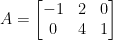 .
.
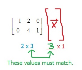
 . To better understand this transformation, we will make a few observations.


 , then:
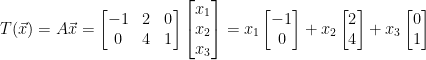
 will be a
  and so any linear combination will also be in
 under T. Then, we would simply “plug” this vector into T.
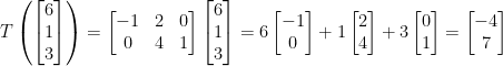
 , the image of
  .
.


 .
.
 . (think: multiply row 2 by 3 and put it back where the original row 2 was)
 next to row 2. To do the actual row operation, we took each value in row 1, multiplied it by –5 and then added it to the corresponding entry in row 2.
  . (the arrow points to where all the work will go)
 in the 2nd equation. If we continued this process and did similar row operations for other variables, then we should be able to eliminate the variables in a way as to see the solution to the underlying system. In fact, this will be exactly what we will study when talking about Gauss Jordan elimination and row reduction.
