Statistics

Finding “and” probabilities with the multiplication rule

The probability of an “and” event, sometimes described as the intersection of two events, can be found using the multiplication rule for probability. In this guide, we will look at this formula and how to use it.

[adsenseWide]

The formula

You can think of this in the following way: to find the “and” probability, find the probability of the first event and multiply it by the probability of the second event given the first. Let’s try it out with an example!

Examples

Example

A bag contains 25 blue and 15 green marbles. Two marbles are selected, one at a time, without replacement. What is the probability both are blue?

To answer this, you must first recognize that “both are blue” is the same as “the first is blue AND the second is blue”. Once you see this is an “and” probability, you can then apply the formula.

\text{P(both blue)} = \text{P(first is blue and second is blue)}

To use the formula, think “probability of the first event times probability of second given the first”. This would give you the following:

\text{P(first is blue and second is blue)} = \text{P(first is blue)}\text{P(second is blue}|\text{first is blue)}

Now we can find each probability. To find the probability the first marble is blue, notice that there are a total of 25 + 15 = 40 marbles and 25 are blue. Therefore:

\text{P(first is blue)} = \dfrac{25}{40}

The next probability, P(second is blue | first is blue), is conditional. So, you must assume that the first marble was already selected and was blue. Since there were 40 marbles originally, there will only be 39 now. And, since there were 25 blue originally, there will only be 24 now.

\text{P(second is blue}|\text{first is blue)} = \dfrac{24}{39}

Plugging these into the formula:

 \text{P(first is blue and second is blue)} = \text{P(first is blue)}\text{P(second is blue}|\text{first is blue)}

 = \left(\dfrac{25}{40}\right)\left(\dfrac{24}{39}\right)

\approx \boxed{0.3846}

The key to this problem was the idea of “without replacement”. This meant that once the marble is selected, it is not put back. This changes the probability that another will be selected since there is 1 marble now gone.

Let’s look at another example that uses the same situation.

Example

A bag contains 25 blue and 15 green marbles. Two marbles are selected, one at a time, without replacement. What is the probability the first is green and the second is blue?

In this example, it is more clear that we have an “and” probability, since it is stated right there in the question! So, we can immediately apply the formula. Again – think “probability of the first times probability of the second given the first”.

\text{P(first green and second blue)} = \text{P(first green)}\text{P(second blue}|\text{first green)}

= \left(\dfrac{15}{40}\right)\left(\dfrac{25}{39}\right)

\approx \boxed{0.2404}

You may notice that we didn’t down each time here. Well, at the start, there are 40 total marbles and 15 are green, so the first probability is 15/40. Then, that marble is removed, so there are 39 remaining. But, since it was green, there are still 25 blue. This gives the conditional probability as 25/39.

Conclusion

This is just the basics of finding probabilities with the multiplication rule. There are also cases where we have independent events (such as selecting WITH replacement) where the formula changes a bit and cases where using the complement may be helpful.

Calculate the mean in minitab

Although it is certainly possible to calculate the mean using the formula (add up the values, divide by how many there are), it is much more efficient and less error prone to use technology. One useful technology tool for calculations and statistics is Minitab. In this article, you will see the steps needed to calculate the mean for any data set in Minitab.

[adsenseWide]

Step 1: Enter the data into minitab

There is no rule that says you have to use the first column, but if you have only one list of data, go ahead and type it into the column C1. We will use the following data set as an example: 16, 14, 15, 17, 16, 16, 18. Do not enter data in the grayed out space right below C1. Instead, enter it only in the white portion of the spreadsheet.

minitab-mean-data-list

While not required, you should also be sure to label the column/data. To do this, highlight the space right below C1 and type in a name. Then, press enter.

minitab-mean-data-list-2

Step 2: Click Stat and select Basic Statistics, then Display Descriptive Statistics…

This is all found at the top menu.

minitab-display-descriptive-statistics

Once you click this, a new menu will come up. Here, double click C1 and then click OK.

minitab-display-descriptive-statistics-menu

After you click OK, the following will display in the part of the screen above your data. In the figure below, the mean is in the red box.

minitab-display-descriptive-statistics-output

Notice that you also get several other values, such as the number of data values (N), the standard deviation (StDEV), as well as the first and third quartiles (Q1 and Q3).

Other considerations

If you already have data in Minitab, or you have multiple variables for which you want to calculate the mean, you can simply double click the correct column in step 2 above. Repeating the step for another column, will then show the basic stats, including the mean, for that column as well.

z-table

The z-table below shows the area under the standard normal curve, to the left of the given z-value.

Table of contents:

  1. z-table for negative z-values
  2. z-table for positive z-values

z-table for negative z-values (area to left)

z 0.00 0.01 0.02 0.03 0.04 0.05 0.06 0.07 0.08 0.09
-0.0 0.5000 0.4960 0.4920 0.4880 0.4840 0.4801 0.4761 0.4721 0.4681 0.4641
-0.1 0.4602 0.4562 0.4522 0.4483 0.4443 0.4404 0.4364 0.4325 0.4286 0.4247
-0.2 0.4207 0.4168 0.4129 0.4090 0.4052 0.4013 0.3974 0.3936 0.3897 0.3859
-0.3 0.3821 0.3783 0.3745 0.3707 0.3669 0.3632 0.3594 0.3557 0.3520 0.3483
-0.4 0.3446 0.3409 0.3372 0.3336 0.3300 0.3264 0.3228 0.3192 0.3156 0.3121
-0.5 0.3085 0.3050 0.3015 0.2981 0.2946 0.2912 0.2877 0.2843 0.2810 0.2776
-0.6 0.2743 0.2709 0.2676 0.2643 0.2611 0.2578 0.2546 0.2514 0.2483 0.2451
-0.7 0.2420 0.2389 0.2358 0.2327 0.2296 0.2266 0.2236 0.2206 0.2177 0.2148
-0.8 0.2119 0.2090 0.2061 0.2033 0.2005 0.1977 0.1949 0.1922 0.1894 0.1867
-0.9 0.1841 0.1814 0.1788 0.1762 0.1736 0.1711 0.1685 0.1660 0.1635 0.1611

z 0.00 0.01 0.02 0.03 0.04 0.05 0.06 0.07 0.08 0.09
-1.0 0.1587 0.1562 0.1539 0.1515 0.1492 0.1469 0.1446 0.1423 0.1401 0.1379
-1.1 0.1357 0.1335 0.1314 0.1292 0.1271 0.1251 0.1230 0.1210 0.1190 0.1170
-1.2 0.1151 0.1131 0.1112 0.1093 0.1075 0.1056 0.1038 0.1020 0.1003 0.0985
-1.3 0.0968 0.0951 0.0934 0.0918 0.0901 0.0885 0.0869 0.0853 0.0838 0.0823
-1.4 0.0808 0.0793 0.0778 0.0764 0.0749 0.0735 0.0721 0.0708 0.0694 0.0681
-1.5 0.0668 0.0655 0.0643 0.0630 0.0618 0.0606 0.0594 0.0582 0.0571 0.0559
-1.6 0.0548 0.0537 0.0526 0.0516 0.0505 0.0495 0.0485 0.0475 0.0465 0.0455
-1.7 0.0446 0.0436 0.0427 0.0418 0.0409 0.0401 0.0392 0.0384 0.0375 0.0367
-1.8 0.0359 0.0351 0.0344 0.0336 0.0329 0.0322 0.0314 0.0307 0.0301 0.0294
-1.9 0.0287 0.0281 0.0274 0.0268 0.0262 0.0256 0.0250 0.0244 0.0239 0.0233

z 0.00 0.01 0.02 0.03 0.04 0.05 0.06 0.07 0.08 0.09
-2.0 0.0228 0.0222 0.0217 0.0212 0.0207 0.0202 0.0197 0.0192 0.0188 0.0183
-2.1 0.0179 0.0174 0.0170 0.0166 0.0162 0.0158 0.0154 0.0150 0.0146 0.0143
-2.2 0.0139 0.0136 0.0132 0.0129 0.0125 0.0122 0.0119 0.0116 0.0113 0.0110
-2.3 0.0107 0.0104 0.0102 0.0099 0.0096 0.0094 0.0091 0.0089 0.0087 0.0084
-2.4 0.0082 0.0080 0.0078 0.0075 0.0073 0.0071 0.0069 0.0068 0.0066 0.0064
-2.5 0.0062 0.0060 0.0059 0.0057 0.0055 0.0054 0.0052 0.0051 0.0049 0.0048
-2.6 0.0047 0.0045 0.0044 0.0043 0.0041 0.0040 0.0039 0.0038 0.0037 0.0036
-2.7 0.0035 0.0034 0.0033 0.0032 0.0031 0.0030 0.0029 0.0028 0.0027 0.0026
-2.8 0.0026 0.0025 0.0024 0.0023 0.0023 0.0022 0.0021 0.0021 0.0020 0.0019
-2.9 0.0019 0.0018 0.0018 0.0017 0.0016 0.0016 0.0015 0.0015 0.0014 0.0014

z 0.00 0.01 0.02 0.03 0.04 0.05 0.06 0.07 0.08 0.09
-3.0 0.0013 0.0013 0.0013 0.0012 0.0012 0.0011 0.0011 0.0011 0.0010 0.0010
-3.1 0.0010 0.0009 0.0009 0.0009 0.0008 0.0008 0.0008 0.0008 0.0007 0.0007
-3.2 0.0007 0.0007 0.0006 0.0006 0.0006 0.0006 0.0006 0.0005 0.0005 0.0005
-3.3 0.0005 0.0005 0.0005 0.0004 0.0004 0.0004 0.0004 0.0004 0.0004 0.0003
-3.4 0.0003 0.0003 0.0003 0.0003 0.0003 0.0003 0.0003 0.0003 0.0003 0.0002
-3.5 0.0002 0.0002 0.0002 0.0002 0.0002 0.0002 0.0002 0.0002 0.0002 0.0002
-3.6 0.0002 0.0002 0.0001 0.0001 0.0001 0.0001 0.0001 0.0001 0.0001 0.0001

z-table for positive z-values (area to left)

z 0.00 0.01 0.02 0.03 0.04 0.05 0.06 0.07 0.08 0.09
0.0 0.5000 0.5040 0.5080 0.5120 0.5160 0.5199 0.5239 0.5279 0.5319 0.5359
0.1 0.5398 0.5438 0.5478 0.5517 0.5557 0.5596 0.5636 0.5675 0.5714 0.5753
0.2 0.5793 0.5832 0.5871 0.5910 0.5948 0.5987 0.6026 0.6064 0.6103 0.6141
0.3 0.6179 0.6217 0.6255 0.6293 0.6331 0.6368 0.6406 0.6443 0.6480 0.6517
0.4 0.6554 0.6591 0.6628 0.6664 0.6700 0.6736 0.6772 0.6808 0.6844 0.6879
0.5 0.6915 0.6950 0.6985 0.7019 0.7054 0.7088 0.7123 0.7157 0.7190 0.7224
0.6 0.7257 0.7291 0.7324 0.7357 0.7389 0.7422 0.7454 0.7486 0.7517 0.7549
0.7 0.7580 0.7611 0.7642 0.7673 0.7704 0.7734 0.7764 0.7794 0.7823 0.7852
0.8 0.7881 0.7910 0.7939 0.7967 0.7995 0.8023 0.8051 0.8078 0.8106 0.8133
0.9 0.8159 0.8186 0.8212 0.8238 0.8264 0.8289 0.8315 0.8340 0.8365 0.8389

z 0.00 0.01 0.02 0.03 0.04 0.05 0.06 0.07 0.08 0.09
1.0 0.8413 0.8438 0.8461 0.8485 0.8508 0.8531 0.8554 0.8577 0.8599 0.8621
1.1 0.8643 0.8665 0.8686 0.8708 0.8729 0.8749 0.8770 0.8790 0.8810 0.8830
1.2 0.8849 0.8869 0.8888 0.8907 0.8925 0.8944 0.8962 0.8980 0.8997 0.9015
1.3 0.9032 0.9049 0.9066 0.9082 0.9099 0.9115 0.9131 0.9147 0.9162 0.9177
1.4 0.9192 0.9207 0.9222 0.9236 0.9251 0.9265 0.9279 0.9292 0.9306 0.9319
1.5 0.9332 0.9345 0.9357 0.9370 0.9382 0.9394 0.9406 0.9418 0.9429 0.9441
1.6 0.9452 0.9463 0.9474 0.9484 0.9495 0.9505 0.9515 0.9525 0.9535 0.9545
1.7 0.9554 0.9564 0.9573 0.9582 0.9591 0.9599 0.9608 0.9616 0.9625 0.9633
1.8 0.9641 0.9649 0.9656 0.9664 0.9671 0.9678 0.9686 0.9693 0.9699 0.9706
1.9 0.9713 0.9719 0.9726 0.9732 0.9738 0.9744 0.9750 0.9756 0.9761 0.9767

z 0.00 0.01 0.02 0.03 0.04 0.05 0.06 0.07 0.08 0.09
2.0 0.9772 0.9778 0.9783 0.9788 0.9793 0.9798 0.9803 0.9808 0.9812 0.9817
2.1 0.9821 0.9826 0.9830 0.9834 0.9838 0.9842 0.9846 0.9850 0.9854 0.9857
2.2 0.9861 0.9864 0.9868 0.9871 0.9875 0.9878 0.9881 0.9884 0.9887 0.9890
2.3 0.9893 0.9896 0.9898 0.9901 0.9904 0.9906 0.9909 0.9911 0.9913 0.9916
2.4 0.9918 0.9920 0.9922 0.9925 0.9927 0.9929 0.9931 0.9932 0.9934 0.9936
2.5 0.9938 0.9940 0.9941 0.9943 0.9945 0.9946 0.9948 0.9949 0.9951 0.9952
2.6 0.9953 0.9955 0.9956 0.9957 0.9959 0.9960 0.9961 0.9962 0.9963 0.9964
2.7 0.9965 0.9966 0.9967 0.9968 0.9969 0.9970 0.9971 0.9972 0.9973 0.9974
2.8 0.9974 0.9975 0.9976 0.9977 0.9977 0.9978 0.9979 0.9979 0.9980 0.9981
2.9 0.9981 0.9982 0.9982 0.9983 0.9984 0.9984 0.9985 0.9985 0.9986 0.9986

z 0.00 0.01 0.02 0.03 0.04 0.05 0.06 0.07 0.08 0.09
3.0 0.9987 0.9987 0.9987 0.9988 0.9988 0.9989 0.9989 0.9989 0.9990 0.9990
3.1 0.9990 0.9991 0.9991 0.9991 0.9992 0.9992 0.9992 0.9992 0.9993 0.9993
3.2 0.9993 0.9993 0.9994 0.9994 0.9994 0.9994 0.9994 0.9995 0.9995 0.9995
3.3 0.9995 0.9995 0.9995 0.9996 0.9996 0.9996 0.9996 0.9996 0.9996 0.9997
3.4 0.9997 0.9997 0.9997 0.9997 0.9997 0.9997 0.9997 0.9997 0.9997 0.9998
3.5 0.9998 0.9998 0.9998 0.9998 0.9998 0.9998 0.9998 0.9998 0.9998 0.9998
3.6 0.9998 0.9998 0.9999 0.9999 0.9999 0.9999 0.9999 0.9999 0.9999 0.9999

Conditional probability – notation and calculation

When finding a conditional probability, you are finding the probability that an event A will occur, given that another event, event B, has occurred. In this article, we will look at the notation for conditional probability and how to find conditional probabilities with a table or with a formula.

[adsenseWide]

Table of contents:

  1. Notation
  2. Conditional probability examples with tables
  3. Conditional probability examples with the formula
  4. Summary

Notation

The image below shows the common notation for conditional probability. You can think of the line as representing “given”. On the left is the event of interest, and on the right is the event we are assuming has occurred.

Conditional probability notation. P(A|B) is read as probability of A given B.

With this notation, you could also use words to describe the events. For example, let’s say you wanted to find the probability someone buys a new car, when you know they have started a new job. This would be represented as:

Image showing conditional probability notation. In this example, we are finding the probability that someone buys a new car given that they started a new job. This is written P(new car | new job)

Example using a table of data

One of the common types of problems you will see uses a two-way table of data. Here, we will look at how to find different probabilities using such a table.

Example

A survey asked full time and part time students how often they had visited the college’s tutoring center in the last month. The results are shown below.

two-way-table-conditional-probability-example

Suppose that a surveyed student is randomly selected.

(a) What is the probability the student visited the tutoring center four or more times, given that the student is full time?

Conditional probability is all about focusing on the information you know. When calculating this probability, we are given that the student is full time. Therefore, we should only look at full time students to find the probability.

Two way table with only the information about full time students highlighted. There were a total of 45 full times students with 8 having visited tutoring four or more times. Therefore P(four or more times |full time) = 8 / 45.

(b) Suppose that a student is part time. What is the probability that the student visited the tutoring center one or fewer times?

This one is a bit more tricky due to the wording. Think of it in the following way:

  • Find: probability student visited the tutoring center one or fewer times
  • Assume or given: student is part time (“suppose that a student is part time”)

Since we are assuming (or supposing) the student is part time, we will only look at part time students for this calculation.

tTwo way table with only part time student data highlighted. In a total of 13 part time students, only 2 went to tutoring one or fewer times. Therefore P(one or fewer times | part time) = 2/13.

(c) If the student visited the tutoring center four or more times, what is the probability he or she is part time?

As above, we need to make sure we know what is given, and what we are finding.

  • Find: probability he or she is part time
  • Assume or given: student visited the tutoring center four or more times (“if the student visited the tutoring center four or more times…”)

For this question, we are only looking at students who visited the tutoring center four or more times.

Two way table with only the data for students who visited tutoring four or more times highlighted. There were 14 such students, and 6 were part time, so P( part time | four or more visits) = 6/14.

As you can see, when using a table, you just need to pay attention to which group from the table you should focus on.

Examples of using the formula to find conditional probability

In some situations, you will need to use the following formula to find a conditional probability.

The conditional probability formula. P(A give B) = P(A and B) divided by P(B).

This formula could actually be used with the table data, though it is often easier to apply in problems similar to the next example.

Example

In a sample of 40 vehicles, 18 are red, 6 are trucks, and 2 are both. Suppose that a randomly selected vehicle is red. What is the probability it is a truck?

We are asked to find the following probability:

\(\text{P(truck}|\text{red)}\)

Applying the formula:

\(\begin{align}\text{P(truck}|\text{red)} &= \dfrac{\text{P(truck and red)}}{\text{P(red)}}\\ &= \dfrac{\tfrac{2}{40}}{\tfrac{18}{40}}\\ &= \dfrac{2}{18}\\ &= \dfrac{1}{9} \approx \boxed{0.11}\end{align}\)

The thinking behind the formula is very similar to the thinking used with the table. For example, notice that what we “know” ends up on the bottom of the fraction. We can also apply this to situations where we are given probabilities and not counts.

Example

A board game comes with a special deck of cards, some of which are black, and some of which are gold. If a card is randomly selected, the probability it is gold is 0.20, while the probability it gives a second turn is 0.16. Finally, the probability that it is gold and gives a second turn is 0.08.

Suppose that a card is randomly selected, and it allows a player a second turn. What is the probability it was a gold card?

This time, we are given the following probabilities:

  • “the probability it is gold is 0.20” -> P(gold) = 0.2
  • “the probability it gives a second turn is 0.16” -> P(second turn) = 0.16
  • “the probability that it is gold and gives a second turn is 0.08” -> P(gold and second turn) = 0.08

We are trying to calculate:

\(\text{P(gold}|\text{second turn)}\)

We can apply the formula to find this probability:

\(\begin{align}\text{P(gold}|\text{second turn)} &= \dfrac{\text{P(gold and second turn)}}{\text{P(second turn)}}\\ &= \dfrac{0.08}{0.16}\\ &= \boxed{0.5}\end{align}\)

You can see that this works out very nicely if you take a moment to write down the information given in the problem. In fact, you could really say that about any real-life/ word problem in math!

[adsenseLargeRectangle]

Summary

Conditional probability is different from other probabilities in that you know, or are assuming, that some other event has already occurred. Therefore when you calculate the probability, you must “narrow your focus” down to the known event. If you are given a table of data, this means focusing only on the row or column of interest. With the formula, this means that the probability of the known event will be in the denominator.

How to find and interpret the z-score

The z-score is a way of counting the number of standard deviations between a given data value and the mean of the data set. In this lesson, we will look at the formula for the z-score, how to calculate it, and a little more closely at this idea of counting standard deviations.

Table of Contents

  1. The formula for the z-score
  2. Calculating and interpreting the z-score
  3. More about interpreting the z-score
  4. Conclusion


[adsenseWide]

The formula

To calculate the z-score, you first find the distance from the mean, and then divide by the standard deviation.

z-score-formula

If we label the value \(x\), we could write the formula as:
z-score-formula-symbols

Calculating and interpreting the z-score

Let’s look at an example to see how to use this formula.

Example

The mean score on a standardized test was 508 with a standard deviation of 42. One test-taker’s score was 590. Find and interpret the z-score for this score.

From the example, we have the following information:

  • The mean is: \(\mu = 508\)
  • The standard deviation is: \(\sigma = 42\)

    Therefore, the z-score is:

    \(\begin{align}z &= \dfrac{x-\mu}{\sigma}\\ &= \dfrac{590 – 508}{42}\\ &= \dfrac{82}{42}\\ &\approx \boxed{1.95}\end{align}\)

    When it comes to interpreting, you should note that by subtracting the mean from a data value, we will get a negative if it is smaller than the mean and a positive if it is larger. So, the sign gives the “direction” away from the mean. By dividing this difference by the standard deviation, we are putting this distance between the mean and the data value in terms of a number of standard deviations. Therefore, we can say:

    “The test-score of 590 is about 1.95 standard deviations above the mean.”

    Interpreting the z-score:
    For a given data value, the z-score gives the number of standard deviations above (positive) or below (negative) the mean.

    More about interpretation

    As you saw above, the value and the sign of the z-score gives you information about the location of the data value. Specifically:

    • A positive z-score means the data value is larger than the mean.

      If a data value has a z-score of 2, that tells us that this data value is 2 standard deviations larger than the mean.

    • A negative z-score means the data value is smaller than the mean.

      If a data value has a z-score of –3.1, then this data value is 3.1 standard deviations smaller than the mean.

    • A z-score of zero means that the data value equals the mean.

      For example, consider a data set with a mean of 50 and a standard deviation of 2. If a data value also is 50, then the z-score is:

      \(\begin{align}z &= \dfrac{x-\mu}{\sigma}\\ &= \dfrac{50 – 50}{2}\\ &= \dfrac{0}{2}\\ &= \boxed{0}\end{align}\)

      This will be the case anytime the mean and the data value are the same.

    [adsenseLargeRectangle]

    Conclusion

    In your study of statistics, you will come across the z-score in a wide variety of settings. For this reason, it is important to make sure you thoroughly understand the ideas discussed here. The best way to do this is to practice the calculation so that it simply becomes second nature! This will help make future topics much easier to understand.

Combinations on the TI83 or TI84 calculator

In counting, combinations are used to find the number of ways a selection can be made, when order doesn’t matter. In this article, we will see how to use a calculator to find combinations. Let’s use an example to see how this works!

[adsenseWide]

You are taking a week-long trip and decide to bring 4 books from your collection of 25 books. How many different groups of 4 books can be selected from your collection?

Here, you only care about which four books are chosen, not the order. Thus, a combination can be used to answer this question: C(25, 4) or “25 choose 4”.

Step 1: Type in the first number

In this case, the first number is 25.

combinations-on-calculator-step1

Step 2: Press [MATH] and go to the PRB menu

You can use the right arrow to select the menu at the top.

combinations-on-calculator-step2

Step 3: Select 3 nCr and press [ENTER]

To select 3: nCr, you can either highlight the 3 or just press the 3 button.

combinations-on-calculator-step3-5

combinations-on-calculator-step3

Step 4: Type the second number and press [ENTER]

We are finding C(25,4), so the second number is 4.

combinations-on-calculator-step4

From this, we see that there are C(25, 4) = 12,650 different groups of 4 books that could be selected. This may seem like the answer is too large, but if you start thinking about how only one book needs to be different for the group of 4 books to be considered a different group, it begins to make more sense.

Other methods for calculating combinations

You can also use the formula to calculate a combination. You can review this, and more about combinations in general, below.

Counting with combinations

Counting with combinations

Combinations are a way of counting how many ways there are to select an object when order doesn’t matter. For example, suppose that you are selecting 3 people from a group of 15 to take a survey. All 3 selected are taking the same survey, and so the order they are selected in isn’t important.

[adsenseWide]

Notation for combinations

Before we get into some examples, it is important to note that there are three common ways to write a combination. Suppose that we are selecting 8 objects from a basket of 20, and the order isn’t important. The number of ways this can be done would be calculated with a combination “20 choose 8”. This can be written as:

notation-for-combinations

Each of these has the same value, they are just different ways of representing the combination. For this article, we will use the third: C(20,8).

Formula for combinations

Combinations can be calculated using either the formula or using a calculator. The formula uses factorials (the exclamation point). Remember that factorials are where you count down and multiply. For example, 4! = 4 x 3 x 2 x 1 = 24.
combinations-formula
Now, we can look at a few examples of counting with combinations.

Examples

For each of these examples, pay close attention to how it is determined that order is not important. Remember that if order was important, we would use permutations instead.

Example

Jacob’s manager asks him to select 3 shifts from the 7 shifts available next week. How many different selections of three shifts are possible?

In this problem, it doesn’t matter which shift Jacob selected first or second, as he will be working the three selected shifts regardless. Therefore, the answer is: C(7,3).

C(7, 3) = \dfrac{7!}{3!(7 - 3)!}

= \dfrac{7!}{3!(4!)}

= \dfrac{7 \times 6 \times 5 \times \overbrace{4 \times 3 \times 2 \times 1}^{\text{cancel}}}{(3 \times 2 \times 1)(\underbrace{4 \times 3 \times 2 \times 1}_{\text{cancel}})}

= \dfrac{7 \times \overbrace{6}^{\text{cancel}} \times 5}{\underbrace{3 \times 2 \times 1}_{\text{cancel}}}

= 7 \times 5

= \boxed{35}

Notice how many terms we were able to cancel out. This will happen with every combination problem, no matter how large the numbers are. Cancelling out at least some of the terms is always nice, as then it is easier to input in the calculator (or, like in the case above, you may not even need a calculator!)

Example

In how many ways can a committee of 6 be selected from a group of 35 students?

When selecting a committee, it is understood that you are simply selecting a group of people to discuss or work on a problem – the order in which they are selected isn’t important since if someone is selected, they are on the committee whether they were selected first or last. Therefore, we can count this using combinations: C(35, 6).

C(35, 6) = \dfrac{35!}{6!(35 - 6)!}

= \dfrac{35!}{6!(29!)}

= \dfrac{35 \times 34 \times 33 \times 32 \times 31 \times 30 \times \overbrace{29 \times 28 \times 27 \times \cdots \times 1}^{\text{cancel}}}{(6 \times 5 \times 4 \times 3 \times 2 \times 1)(\underbrace{29 \times 28 \times 27 \times \cdots \times 1}_{\text{cancel}})}

= \dfrac{35 \times 34 \times 33 \times 32 \times 31 \times \overbrace{30}^{\text{cancel}}}{(\underbrace{6 \times 5}_{\text{cancel}} \times 4 \times 3 \times 2 \times 1)}

= \dfrac{35 \times 34 \times 33 \times 32 \times 31}{4 \times 3 \times 2 \times 1}

= \boxed{1\,623\,160}

This number may seem very large, but you would be surprised how many different choices there are when the group you are selecting from is large. It is very common in counting problems to come across very large answers like this.

Combinations on the calculator

You can also use a calculator to calculate combinations. To see how to use a TI83 or 84 calculator for this, see the article below.

Combinations on the TI83 or TI84 calculator

t-test for the mean using a TI83 or TI84 calculator (p-value method)

Do people tend to spend more than 2 hours on a computer every day? Can you say that the mean age of a college freshman in your state is not 18 years old? These are the types of questions that can be answered using collected data and a t-test for the mean. In this guide, you will see how you can use a TI83 or TI84 calculator to perform this test using the p-value method.

[adsenseWide]

We will use an example to see how this process works. For this example, assume that the requirements for a hypothesis test for the mean are met (randomly selected sample, independent observations, large population size).

Example: performing a t-test on the calculator

Suppose that a marketing firm believes that people who are planning to purchase a new TV spend more than 7 days researching their purchase. They conduct a survey of 32 people who had recently purchased a TV and found that the mean time spent researching the purchase was 7.8 days with a standard deviation of 3.9 days. At a significance level of 0.05, does this survey provide evidence to support the firm’s belief?

Step 1: Write the null (H_0) and alternative (H_a) hypotheses

The alternative hypothesis is a statement about what you are testing. Here, you are testing the firm’s belief that the mean time spent is more than 7 days. In hypothesis testing, we are trying to understand a population value using a sample, so your hypothesis should be in terms of the population parameter. In this case, that is the population mean, \mu.


\text{mean time spent is more than 7 days} \rightarrow H_a: \mu > 7

The null hypothesis is the equality* statement using the same value:


H_0: \mu = 7

Putting these together, the null and alternative hypotheses are:


H_0: \mu = 7\\ H_a: \mu > 7

(*In some books, they use the statement that is the opposite of H_a for the null hypothesis. Here, that would be H_0: \mu \leq 7. Make sure you use the form preferred in the class you are taking!)

Step 2: Calculate the p-value using your calculator and the correct test

A t-test is used here since we have a big enough sample, and the population standard deviation (\sigma) is unknown. (We only have the standard deviation from the sample: s = 3.9.) Note that if we knew the population standard deviation, we would use a z-test instead.

1. Press [STAT] then go the the TESTS menu.

tests-menu-ti83-or-ti84

2. Select “2. T-test”. Make sure that you highlight Stats and press [ENTER] if your screen looks different from this.

t-test-menu-ti83-or-ti84

3. Enter the values and select the correct tail for the test.

t-test-example-ti83-ti84

4. Highlight Calculate and press [ENTER].

t-test-ti83-ti84-example-2

Step 3: Compare the p-value to the significance level alpha (\alpha) and make your decision

From the last line of the calculator, \text{p-value} \approx 0.1274. Further, the last part of the problem stated “At a significance level of 0.05, does this survey provide evidence to support the firm’s belief?”. Therefore, \alpha = 0.05.

To make the decision, use the decision rule:

decision-rule-p-value

In this problem:

t-test-example-decision

Step 4: Interpret your decision in terms of the problem

If you fail to reject H_0, then you are saying there is not enough evidence for H_a. Remember for this problem:


H_0: \mu = 7\\ H_a: \mu > 7

So, we are saying that there is not enough evidence that the population mean is greater than 7. In context, we are saying:

This sample does not provide evidence that the mean time spent researching a new TV purchase is more than 7 days.

Although our sample mean was in fact larger than 7, it wasn’t quite enough to suggest that this is true for the entire population. Remember, in hypothesis testing, that is what we are trying to determine – is the sample enough to say that the hypothesis holds for the entire population?

Binomial probabilities – examples (calculator)

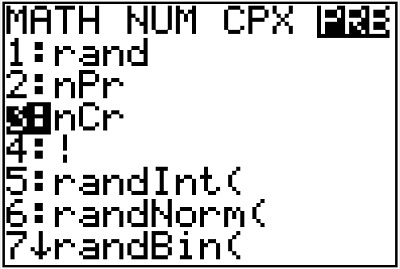
Once you have determined that an experiment is a binomial experiment, then you can apply either the formula or technology (like a TI calculator) to find any related probabilities. In this lesson, we will work through an example using the TI 83/84 calculator. If you aren’t sure how to use this to find binomial probabilities, please check here: Details on how to use a calculator to find binomial probabilities.

[adsenseWide]

Example

A student is taking a multiple choice quiz but forgot to study and so he will randomly guess the answer to each question. There are a total of 12 questions, each with 4 answer choices. Only one answer is correct for each question.

Verifying the experiment is binomial

We know that this experiment is binomial since we have \(n = 12\) trials of the mini-experiment “guess the answer on a question”. There are two outcomes: “guess correctly”, “guess incorrectly”.

If we treat a success as guessing a question correctly, then since there are 4 answer choices and only 1 is correct, the probability of success is:

\(p = \dfrac{1}{4} = 0.25\)

Finally, since the guessing is random, it is reasonable to assume that each guess is independent of the other guesses.

Calculating probabilities

We will let \(X\) represent the number of questions guessed correctly. Let’s now use this binomial experiment to answer a few questions.

(a) Find the probability that he answers 6 of the questions correctly.

This is asking for the probability of 6 successes, or \(P(X = 6)\). For finding an exact number of successes like this, we should use binompdf from the calculator.

For this problem, \(n = 12\) and \(p = 0.25\). Therefore:

\(\begin{align} P(X=6) &= \text{binompdf(12,0.25,6)} \\ &\approx \boxed{0.0401}\end{align}\)

(b) Find the probability that he correctly answers 3 or fewer of the questions.

The probability of 3 or fewer successes is represented by \(P(X < 3)\). Anytime you are counting down from some possible value of \(X\), you will use binomcdf. binomcdf-ti84-84

\(\begin{align}P(X < 3) &= \text{binomcdf(12, 0.25, 3)} \\ &\approx \boxed{0.6488}\end{align}\)

It isn’t looking good. This is a pretty high chance that the student only answers 3 or fewer correctly!

(c) Find the probability that he correctly answers more than 8 questions.

This probability is represented by \(P(X > 8)\). To understand how to find this probability using binomcdf, it is helpful to look at the following diagram.

possible-values-more-than-8

This shows all possible values of \(X\) with the values which would represent “more than 8 successes” highlighted in red. To calculate this, we could do the binompdf of 9, the binompdf of 10, the binompdf of 11, and the binompdf of 12 and add them all together. But, this would take quite a while. Instead, we could use the complementary event.

possible-values-more-than-8-the-complement

Recall that \(P(A)\) is \(1 – P(A \text{ complement})\). So, we can write:

\(\begin{align} P(X > 8) &= 1 – P( X < 8) \\ &= 1 - \text{binomcdf(12, 0.25, 8)}\\ &\approx \boxed{3.9 \times 10^{-4}}\end{align}\)

This is a very small probability. Looks like the random guessing probably won’t pay off too much.

(d) Find the probability that he correctly answers 5 or more questions.

This probability is represented by \(P(X \geq 5)\). Using our diagram:

5-or-more-possible-values-of-X

Again, since this is asking for a probability of > or \(\geq\);, and the CDF only counts down, we will use the complement. Notice that the complementary event starts with 4 and counts down. So, we will use 4 in the CDF.

\(\begin{align}P(X \geq 5) &= 1 – P(X < 5)\\ &= 1 - \text{binomcdf(12, 0.25, 4)}\\ &\approx \boxed{0.1576}\end{align}\)

(e) Find the probability that he correctly answers fewer than 2 questions.

This is asking for \(P(X < 2)\). smaller-than-2

Since this is counting down, we can use binomcdf. But, the event “fewer than 2” does not include 2. So, we will put 1 into the cdf function.

\(\begin{align} P(X < 2) &= \text{binomcdf(12, 0.25, 1)}\\ &\approx \boxed{0.1584}\end{align}\)

(e) Find the probability that he correctly answers between 5 and 10 questions (inclusive) correctly.

Since this is inclusive, we are including the values of 5 and 10. That is, we are finding \(P(5 \leq X \leq 10)\).

between-5-and-10

Remember, you can always find the PDF of each value and add them up to get the probability. Here however, we can creatively use the CDF. Recall that the CDF takes whatever value you put in and adds the PDFs for each value starting with that number all the way down to zero. If we find the CDF of 10, it will add the PDFs of 10, 9, 8, 7, 6, 5, 4, 3, 2, 1, and 0.

between-5-and-10-cdf-10

This will include all the values below 5, which we don’t want. So, we will subtract them out!

between-5-and-10-cdf-10and4

This will leave exactly the values we want:

\(\begin{align}P(5 \leq X \leq 10) &= \text{binomcdf(12,0.25,10)} – \text{binomcdf(12,0.25,4)}\\ &\approx \boxed{0.1576}\end{align}\)

Interesting observation

Did you notice that two of our answers were really similar? We found that:

\(\begin{align}P(X \geq 5) &= 1 – P(X < 5)\\ &= 1 - \text{binomcdf(12, 0.25, 4)}\\ &\approx \boxed{0.1576}\end{align}\)

and

\(\begin{align}P(5 \leq X \leq 10) &= \text{binomcdf(12,0.25,10)} – \text{binomcdf(12,0.25,4)}\\ &\approx \boxed{0.1576}\end{align}\)

What is going on here?

Well, these probabilities aren’t exactly the same. The first is actually 0.1576436761 while the second is 0.1576414707. These are certainly very close though! The tiny difference is because \(P(X \geq 5)\) includes \(P(X = 11)\) and \(P(X = 12)\), while \(P(5 \leq X \leq 10)\) does not.

Further, \(P(X = 11)\) represents the probability that he correctly answers 11 of the questions correctly and latex \(P(X = 12)\) represents the probability that he answers all 12 of the questions correctly. Both events are very unlikely since he is guessing! In fact:

\(\begin{align}P(X = 11) &= \text{binompdf(12,0.25,11)} \\ &\approx \boxed{2.14 \times 10^{-6}}\end{align}\)

and

\(\begin{align} P(X = 12) &= \text{binompdf(12,0.25,12)} \\ &\approx \boxed{5.96 \times 10^{-8}}\end{align}\)

Since these are so tiny, including them in the first probability only increases the probability a little bit. Rounding to 4 decimal places, we didn’t even catch the difference.

[adsenseLargeRectangle]

Summary

The only reason we were able to calculate these probabilities is because we recognized that this was a binomial experiment. This fact allowed us to use binompdf for exact probabilities and binomcdf for probabilities that included multiple values. Just remember – binomcdf is cumulative. It adds up PDFs for the value you put in, all the way down to zero. Using this, you can find pretty much any binomial probability as long as you use something like the diagrams we drew above to keep track of the needed values.

Binomial experiments

One tough part of probability is recognizing which rule to use and when. Binomial probabilities may seem difficult, but in a way they are nice because there is a set formula to use. However, to know to use this formula, you must first determine whether or not the situation you are working with represents a binomial experiment. We will see how to do this below.

[adsenseWide]

How to determine if an experiment is binomial

A binomial experiment is any probability experiment where the following four properties hold.

  • The experiment consists of a series of n trials.

    You can think of each trial as a “mini-experiment”. For example, if you flip a coin 10 times, there are 10 mini-experiments. The mini-experiment, or trial, is “flip a coin”. The number of trials is usually labelled “n”.

  • Each trial has two outcomes.

    We call these two outcomes “success” and “failure”, but really a success is simply the label for whatever we are counting. In the coin flip example, we could call heads a success and tails a failure.

  • There is a fixed probability of success for each trial.

    For an experiment to be a binomial experiment, we must have that the probability of success doesn’t change from trial to trial. Using a coin flip again (flipping a coin multiple times is a classic binomial experiment example), the probability of heads stays the same on each flip. The probability of success is usually labelled “p”, while the probability of failure is usually labelled “q”.

  • Each trial is independent of the others.

    It is said that a coin “has no memory”. That is, regardless of whether or not the coin landed on tails 100 times in a row, the probability of heads or tails remains the same. This idea of independence is needed in order to classify a probability experiment as being a binomial experiment.

Examples of binomial experiments

An important skill in a probability and statistics course is to be able to identify binomial experiments. So, we will look at a couple of examples and see how they fit the rules listed above.

Example

Data collected from a website shows that 39% of visitors use internet explorer. Randomly select 6 visitors and record how many use internet explorer.

  • fixed number of trials
    We can view this experiment as 6 repetitions of the mini-experiment “determine if a visitor uses internet explorer”. Thus, there are n = 6 trials.

  • two outcomes
    There are two possible outcomes to each trial: the visitor uses internet explorer or they do not use internet explorer.

  • fixed probability of success
    A success is often based on what you are recording. Here, we are interested in how many visitors use internet explorer. Given the data, we can assume that for any visitor, the probability they use internet explorer is 39%. So, p = 0.39.

  • independence
    There is no reason to assume that the probability one person uses internet explorer is affected by the fact that another person uses it. Thus, we do have independence.

Given the above information, we can say that this is a binomial experiment.

Example

Roll a single 6 sided fair die 14 times. Record the number of times a 5 comes up.

  • fixed number of trials
    We can view this experiment as 14 repetitions of the mini-experiment “roll a 6 sided fair die”. Thus, there are n = 14 trials.

  • two outcomes
    There are two possible outcomes based on what we are recording: “a 5 comes up”, “a 5 does not come up”.

  • fixed probability of success
    The probability a 5 comes up is 1/6. This is the same for each die roll. Thus, p = 1/6.

  • independence
    Die rolls, like coin flips, are always independent.

Once again, since these properties hold, we have a binomial experiment.

Why is this useful?

It may seem really academic to say that an experiment is binomial or not. However, it is actually very useful when it comes to calculating probabilities. Knowing an experiment is binomial allows us to use a formula or technology to find the probability of any number of successes occurring. To see this, take a look at this binomial probability example.